A Note on Keynes’ General Theory

The basic aggregate model summarized by Keynes in Chapter 18 of The General Theory of Employment, Interest, and Money is derived from the implicit general equilibrium model that underlies Keynes’ general theory. It is argued that when these models are viewed from the perspective of the simple dynamics of supply and demand it becomes clear that the methodology of Keynes is Marshallian rather than Walrasian and that this makes Keynes’ methodology causal and dynamic whereas the Walrasian methodology is, at best, descriptive and incapable of meaningful causal or dynamic analysis.

Keynes did not present his general theory as a system of simultaneous equations. That was done by J. R. Hicks, A. H. Hansen, P. A. Samuelson, D. Patinkin, and countless other Keynesians. Their approach was Walrasian, and as a result of their efforts a Walrasian revolution in the name of Keynes took place in economics following Keynes’ publication of The General Theory of Employment, Interest, and Money. [Clower; Leijonhufvud] This revolution took Keynes’ name in spite of the fact that Keynes was a protégé of Marshall, not Walras. Keynes emphatically rejected the kind of mathematical approach embraced by the Walrasians that ignore the problems imposed by empirical reality:

This is the methodology of Marshall, not of Walras, and Keynes spent his entire life applying this methodology in an attempt to discover the causal relationships that drive the economic system through time. In so doing, among many other things, it became clear to him that 1) the ultimate justification for production is to satisfy the demands of consumers, 2) the true causal variables in a market economy in which the processes of production take time are expectations with regard to the future, 3) rates of interest are a purely monetary phenomena determined by the supply and demand for liquidity as the prices of assets adjust to equate wealth-holder demands for assets to the existing stocks of assets, 4) monetary policy is limited in its ability to stimulate the economy by the propensities of wealth holders with regard to their demands for liquidity, 5) once rates of interest have reached the lower bounds set by the propensities of wealth holders the level of economic activity is determined by the propensity to consume and the demand for investment goods, and 6) since the demand for investment goods is ultimately determined by expectations with regard to future consumption, and since expectations with regard to future consumption are largely determined by current consumption, the level of economic activity must be largely determined by current consumption and, ultimately, by the way in which current consumption changes over time. [See Blackford (2016)]

Even though these arguments and this conclusion stand at the very core of Keynes’ general theory [Blackford (2016)], this way of looking at the economic system was not taught or even acknowledged in graduate schools when I was in academia, and I suspect is not taught or acknowledged in graduate schools to this day. Instead, graduate students were taught the Walrasian paradigm with tâtonnement/recontract dynamics while the Marshallian paradigm from which the dynamics of Keynes is drawn was pretty much ignored other than in undergraduate courses.

It is obvious, or at least it should be obvious, that something is wrong here. In point of fact, neither households nor firms are constrained in their choices in the real world by a Walrasian budget constraint at the points in time at which a choice must be made. They are constrained by a) the value and liquidity of their assets, b) the availability of sellers of goods at various prices, c) the availability of buyers of goods at various prices, and d) in their access to credit. They have no choice but to be guided by their expectations with regard to the future, as Keynes insisted, but they are not constrained in the present by what actually happens in the future. The rate at which decision-making units receive income at the point in time at which a decision must be made has no way of affecting that decision other than through its effect on expectations as any consumer who has ever purchased a home, a car, or has simply walked the aisles of a supermarket knows implicitly, and as any businessman who has ever had to meet a payroll knows implicitly as well. These are simple, empirical facts, and yet the Walrasian budget constraint presupposes a) that all prices, quantities, and incomes are known at the time a choice must be made, b) that all choices are made simultaneously, and c) that those choices are constrained by income. This sort of thing can correspond to actual behavior only in a world in which expectations are always realized and markets always clear, that is, when the system is in static equilibrium. [Clower] The Walrasian budget constraint has no relevance at all when the system is not in static equilibrium. [Blackford (1975; 1976)] There is no mystery about this. It is well known that Walrasian dynamics is empirically irrelevant by virtue of its reliance on the mythical auctioneer of the Walrasian tâtonnement/recontract assumption. [Jaffe]

The real mystery is why so many economists have invested so much time and energy over the years trying to prove that Keynes is wrong as they ignore Marshall and attempt to force Keynes into a Walrasian mold. This is especially so in view of the fact that virtually nothing Keynes actually said in The General Theory makes sense when viewed from the perspective of the Walrasian paradigm and can only be understood from the perspective of Marshall.

The purpose of this note is to explain the methodology used by Keynes throughout The General Theory in terms of the simple dynamics of supply and demand on which it is based—a dynamics that has been taught, I believe, in every principles course in economics throughout the world for well over one hundred years—and to contrast this methodology with that embodied in the Walrasian paradigm. It is hoped that by highlighting the fundamental difference between these two methodologies it might make it possible for economists to better understand the nature of Keynes’ general theory, and, even more important, to better understand how the economic system actually works so as to make mainstream economic theory more empirically relevant.

I. The Simple Dynamics of Supply and Demand

The simple dynamics of supply and demand is generally explained in terms of a partial-equilibrium analysis of a competitive market characterized by an upward sloping supply schedule and downward sloping demand schedule as shown in the diagram in Figure 1—a diagram that any student who has taken a principles of economics class should recognize immediately and understand implicitly.

It illustrates a situation in which a market begins with an equilibrium price P and quantity Q as determined by the intersection of the initial supply schedule S and demand schedules D and then experiences a ceteris paribus increase in supply that shifts the supply schedule from S to S’. This results in an excess supply at the original equilibrium price equal to the difference between Q and Q” which is the quantity in excess of the amount suppliers are willing to sell over the amount buyers are willing to buy at the original market price P. Since this is a competitive market we can expect suppliers to attempt to increase their output at the original price P and competition among suppliers and demanders to bid down the market price in an attempt to increase their sales and purchases. This competition will, in turn, cause the price to fall and cause the quantity produced and sold in the market to increase until the new equilibrium price P’ and quantity Q’ are achieved at the intersection of the initial demand curve D and the new supply curve S’. At this price and quantity, and only at this price and quantity, will it be possible for suppliers to sell all they are willing to sell and demanders to purchase all they are willing to purchase, and there is no reason for the market price or quantity produced and exchanged in the market to change.

This example of the simple dynamics of supply and demand assumes a competitive market, but even if the market is not competitive we can still use the methodology of this example to examine the cause and effect implications of the various kinds of noncompetitive phenomena with which we are confronted as anyone who has taken an undergraduate intermediate microeconomics class well knows. In addition, since all of the non-price factors that affect the willingness to buy and sell are assumed to be subsumed in the functional form of the supply and demand schedules, the usefulness of this methodology is not limited to a single market in a ceteris paribus situation. This simple paradigm can be used to analyze the effects of the price and quantity changes in the given market on other markets (e.g., the markets for substitutes and compliments) and the feedback effects on the given market from the subsequent price and quantity changes in those other markets, ad infinitum, if one wishes, until a short-run or general equilibrium is reached. Even when the assumptions underlying the analysis are not strictly met, the overall contribution of the metaphorical application of this kind of analysis to the understanding of practical economic problems is such that it is an indispensable part of the economist’s way of thinking. One might even say: “This is the nature of economic thinking.” In any event, this was the nature of Keynes’ thinking as he wrote The General Theory.

It is my view that the methodology embodied in the simple example presented in Figure 1 is the single most powerful analytical tool available to economists as a guide to understanding how the economic system works. There are two reasons for this:

First, this methodology explains the determination of prices and quantities and what will cause prices and quantities to change in terms of the behavior of those decision-making units—suppliers and demanders—who actually have the power to determine and change the prices and quantities bought and sold in the market.

Second, since there must be a change in either supply or demand before a change in price or quantity can occur within this methodology it is possible to examine individual markets, prices, and quantities in sequential order which makes it is possible to establish the temporal order in which events must occur.

These two characteristics of the simple supply and demand methodology make it possible to separate cause and effect and, thus, to provide a causal explanation of dynamic behavior within this context.

The situation is fundamentally different within the context of the Walrasian paradigm. Since everything is assumed to change simultaneously if anything changes, it is impossible to establish the temporal order in which events must occur within this paradigm. As a result, it is only possible to provide a mythical analysis of dynamic behavior within the context of the Walrasian paradigm by way of the mythical auctioneer of the tâtonnement/recontract assumption.

II. The Marshallian Roots of Keynes’ General Theory

In writing his Treatise on Money Keynes discovered that it is impossible to provide a logically consistent, causal explanation of the way in which the rate of interest would change in response to a change in the saving or investment schedule in a ceteris paribus situation in which income and the supply and demand for money are given. That meant that it was not enough to know what was happening to the saving and investment schedules to be able to predict what would happen to the rate of interest. He also had to know what was happening to income and the supply and demand for money because in the absence of a change in income or the supply or demand for money there was no way to explain why the rate of interest would change. What this meant was that he could not use the simple methodology of supply and demand to give a causal explanation of how the rate of interest was determined or to establish the temporal order in which events must occur with regard to the rate of interest if he assumed that the rate of interest is determined by savers and investors. At the same time he discovered that there is a reason for the rate of interest to change in a ceteris paribus situation in which income and the supply of money are given if there is a change in “hording,” that is, if there is a change in the demand for money. [See Keynes (1930, pp. 145-6); and Blackford (1983; 1986; 1987; 2016)]

In pursuing this problem on the way to his general theory Keynes came to realize that, unlike the case for savers and investors, it is possible to give a logically consistent, causal explanation of the way in which suppliers and demanders for money change the rate of interest in a ceteris paribus situation in response to a change in the supply or demand for money. Thus, Keynes concluded that the only way to make sense out of saving, investment, income, and the rate of interest in terms of cause and effect that establishes the temporal order in which events must occur is to assume that the rate of interest is determined by the supply and demand for money and that investment is determined by supply and demand in the markets for investment goods. [See Blackford (1983; 1986; 1987; 2016)] The relevance of these conclusions to Keynes’ general theory can be seen by specifying the kinds of dynamic market adjustment equations that are implicit in the idea that the rate of interest is determined by the supply and demand for money and that investment is determined by the supply and demand in the markets for investment goods.

III. Implicit Adjustment Equations in Keynes' General Theory

In specifying the market adjustment equations implicit in the assumption that the rate of interest is determined by the supply and demand for money it is assumed that the rate at which suppliers and demanders for money interact to adjust the rate of interest (R) to equate the quantities of money supplied and demanded (M^s and M^d) is a function of the excess demand for money (M^d – M^s):

and that suppliers and demanders of money interact in such a way as to adjust the actual stock of money in existence (M) toward the short side of the market, that is, toward the quantity demanded when there is a surplus and toward the quantity supplied when there is a shortage: 0F[1]

where dR and dM denote the time derivative operator d (=d/dt) applied to R and M, respectively, and the functions f ^r and f ^m (as well as the time derivative functions specified below) are assumed to increase monotonically through the origin. Equations (1) and (2) simply formalize the idea that when M^d and M^s are not equal to M, demanders and suppliers in the money markets will interact in such a way as to cause R to adjust so as to reduce the difference between the supply and demand for money and cause M to adjust toward the short side of the market.

In specifying the market-adjustment equations implicit in Keynes’ second conclusion, that investment is determined by the supply and demand for investment goods in the markets for investment goods, it is assumed that the rate at which suppliers and demanders for investment goods adjust the price of investment goods (Pⁱ) to equate the quantities supplied (I^s) and demanded (I^d) is a function of the excess demand for investment goods (I^d - I^s):

and that suppliers and demanders of investment goods adjust the actual rate of investment (I) toward the short side of the market:

Again, this specification simply states that, when I^d and I^s are not equal to I, demanders and suppliers in the investment-goods markets will interact in such a way as to cause Pⁱ to adjust to reduce the difference between the supply and demand for investment goods and will cause I to adjust toward the short side of the market.

Next we assume that the suppliers and demanders for labor in the investment-goods industries adjust wages in those industries (Wⁱ) by a function of the difference between the supply and demand for labor in the investment-goods industries (N^is and N^id) and the actual level of employment in those industries (Nⁱ) toward the short side of the market:

(6) dNⁱ = f ⁿⁱ(N^id – Nⁱ) if N^id ≤ N^is
= f ⁿⁱ(N^is – Nⁱ) if N^id > N^is.

Having specified (1) through (6) all that is needed to complete the model is to specify a comparable set of adjustment equations for the consumer-goods industries:

(10) dN^c = f ^nc(N^c^d – N^c) if N^c^d ≤ N^c^s = f ^nc(N^c – N^c^s) if N^c^d > N^c^s.

where the form of (7) through (10) is identical to that of (3) through (6), the only difference being the substitution of the c and C notation in (7) through (10) for the i and I notation in equations (3) through (6) to indicate that the corresponding adjustment equations refer to the consumer-goods markets rather the investment-goods markets. [2]

IV. The Structure of Keynes’ General Equilibrium Model

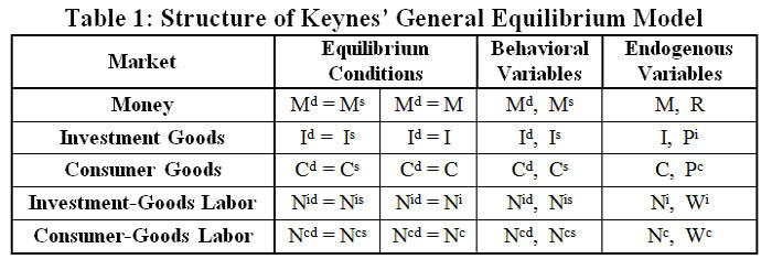
The adjustment equations (1) - (10) define the way in which changes in the endogenous variables of the model are determined in five markets: money, investment goods, investment-goods labor, consumer goods, and consumer-goods labor. Since these adjustment functions are assumed to increase monotonically through the origin, the system is in equilibrium in the sense that there is no reason for any variable to change when all of the independent variables in (1) – (10) are equal to zero. This gives us five markets with ten equilibrium conditions which contain ten behavioral variables and ten endogenous variables as summarized in Table 1.

This table shows the mathematical structure of the general equilibrium model that underlies Keynes’ general theory. Since the behavioral variables in this model are quantities supplied and demanded, economic theory tells us they are functions of all of the endogenous variables. Thus, if the set of Marshallian supply and demand equations that define the behavioral variables in this model are well behaved (a rather heroic assumption within this context given the fact that the purpose of The General Theory is to explain why this set of equations is not that well behaved) the supply and demand equations which define the quantities supplied and demanded can presumably be substituted into the equilibrium conditions and solved for the endogenous variables in terms of the exogenous variables. Thus, all of the equilibrium values of the endogenous variables in this model are, in principle, determined within this system by the behavioral relationships embodied in the supply and demand equations implicit in Table 1.

The fundamental difference between the structure of this model and that of the Walrasian paradigm taught in graduate schools is that the behavioral equations of this model are assumed to be Marshallian supply and demand functions rather than Walrasian supply and demand functions. Marshallian supply and demand functions are derived from the presumed optimizing behavior of decision-making units as they interact in markets, just as Walrasian supply and demand functions are derived. The difference is that the Marshallian functions are derived in a way that attempts to isolate those factors that have a direct influence on the choices of decision-making units without assuming these choices are constrained by an arbitrarily defined Walrasian budget constraint. They are derived by observing the actual choices available to decision-making units in markets, hypothesizing with regard to the motivations of these units, and then reasoning through the logical implications of what the actual choices available to decision-making units and their motivations imply with regard to their willingness to buy and sell. [see Marshall and Keynes and cf. Clower and Blackford (1975; 1976)]

V. The Structure of Keynes’ Aggregate Model

Keynes provided a summary of the given factors and independent and dependent variables in the analytical framework he developed throughout The General Theory at the beginning of Chapter 18 and then summarized the basic form of the short-run, aggregate model embodied in this framework:

Since Keynes’ aggregate model makes use of only two measures of quantity—money and the labor-unit defined as “an hour's employment of ordinary labour” where he assumes that special labor is paid in proportion to its productivity relative to ordinary labor [Keynes (1936, p.41)]—we can specify the dynamic adjustment mechanisms of Keynes’ general theory that apply to the elementary aggregate model described in this paragraph in terms of these units, first by specifying the aggregate real income (output) measured in the wage-unit (Y_w) by dividing the individual values of consumption goods (P^cC) and investment goods (PⁱI) produced in Table 1 by the wage-unit (W) then summing to obtain:

We can then specify the aggregate demand for output (Y^dw) in terms of the aggregate demand for consumption goods (C^dw) and investment goods (I^dw), all measured in wage-units, as being given by:

which embodies “the psychological propensity to consume” and his investment demand function:

which embodies “the psychological expectation of future yield from capital-assets.”

The “the psychological attitude to liquidity” is embodied in Keynes’s liquidity preference function implicit in the general equilibrium model outlined in Table 1, that is, is embodied in the function that defines the demand for money measured in wage units (m^dw). We can specify this function in terms of wage-units as:

There are four endogenous aggregate variables (Y_W, C_W, I_W, and R) to be determined in this model in terms of the given “independent variables.” The dynamic adjustment equations for these four variables that are implicit in Keynes’ general theory are given by:

where M_w is “the quantity of money as determined by the action of the central bank” measured in wage-units.

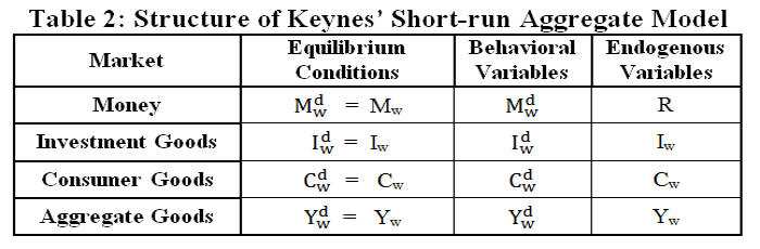
As with the general equilibrium model specified above, the adjustment equations (16) - (19) define the way in which changes in the endogenous variables of the model are determined, except that here we are examining only four aggregate markets: money, investment goods, consumer goods, and the aggregate of the investment and consumer goods markets. Again, since these adjustment functions are assumed to increase monotonically through the origin, the system is in equilibrium in the sense that there is no reason for any variable to change when all of the independent variables in (16) – (19) are equal to zero. This gives us four markets with four equilibrium conditions which contain four behavioral variables and four endogenous variables as summarized in Table 2. 2[3]

This table shows the mathematical structure of the basic short-run aggregate model described by Keynes in the passage quoted above, and since the behavioral variables in this model are functions of the aggregated quantities supplied and demanded (measured in wage-units) in the underlying general equilibrium model, economic theory tells us that the aggregate quantities supplied and demanded are functions of the set of endogenous variables. Thus, if the set of aggregate equations that define the behavioral variables in this model are well behaved the supply and demand equations which define the quantities supplied and demanded can presumably be substituted into the equilibrium conditions and solved for the endogenous variables in terms of the exogenous variables. Thus, all of the equilibrium values of the endogenous variables in this model are, in principle, determined within this system by the behavioral relationships defined by the aggregate equations given by equations (12) through (15).

Since the behavioral variables and adjustment equations in this aggregate model are derived from the behavioral variables and adjustment equations of the general equilibrium model it is possible to apply the same simple methodology of supply and demand to establish the temporal order in which events must occur within the aggregate model outlined in Table 2 that applies to the general equilibrium model outlined in Table 1. This makes it possible to undertake a causal analysis of dynamic behavior within context of the aggregate model, just as in the general equilibrium model, “by isolating the complicating factors one by one” and then going “back on ourselves and allow[ing], as well as we can, for the probable interactions of the factors amongst themselves” which is what Keynes did with this basic aggregate model in excruciating detail throughout The General Theory of Employment, Interest, and Money.

VI. Summary and Conclusion

When viewed from the prospective of the simple dynamics of supply and demand, the structure of the models outlined in Tables 1 and 2 provides a logically consistent framework within which it is possible to examine the fundamental questions of economics that Keynes addressed in The General Theory with regard to how the economic system functions and why it fails to function in the way mainstream economists believe it should function—the kind of analysis that is empirically relevant to the kinds of economic problems we actually face in the real world. These models also provide a logically consistent framework in which a general theory can be developed in that they not only include the monetary sector of the economy, but, at the same time, all prices and quantities are determined by way of the fundamental constructs of supply and demand which lies at the core of Marshall’s theory of value. And the key to the structure of this framework is Keynes’ insight with regard to the fact that the rate of interest is a purely monetary phenomenon, causally determined by the supply and demand for money, not by saving and investment. 3F[4]

Keynes achieved this insight through the methodology of Marshall, namely, by observing the actual choices available to decision-making units in markets, hypothesizing with regard to the motivations of those units, and reasoning through the logical implications of what the available choices and motivations imply with regard to the determination of prices and quantities that are actually observed in markets. He did not achieve this insight by creating abstract mathematical models of representative households and firms in the Walrasian tradition and then attributing the properties of the part to the whole. And it is worth reemphasizing here that the methodology Keynes applied to the models summarized in Tables 1 and 2 is causal and dynamic, not simply because the model is derived from an abstract specification of dynamic adjustment mechanisms, but because these mechanisms are defined in terms of the fundamental Marshallian concepts of quantities supplied and quantities demanded. This makes it possible to use the simple methodology of supply and demand to establish the temporal order in which events must occur and, thus, to provide a causal analysis of dynamic behavior in terms of the choices of those decision-making units that actually have the power to effect that behavior both when the system is in equilibrium and when it is not. [cf. Clower and Blackford (1975; 1976)]

When the models outlined in Tables 1 and 2 are viewed from the perspective of the Walrasian paradigm—all prices and quantities always known, expectations always realized, markets always in equilibrium—the result is an analytic framework that is, at best, descriptive, static, and incapable of meaningful causal or dynamic analysis. When viewed from the perspective of the Marshallian paradigm the result is an analytic framework in which a logically consistent, causal analysis of dynamic behavior is possible, the kind of causal analysis of dynamic behavior undertaken by Marshall throughout his Principles of Economics and by Keynes throughout The General Theory of Employment, Interest, and Money.

This methodology may not be mathematically elegant, which undoubtedly accounts for its lack of appeal to academic economists, but it does make it possible to separate cause and effect and to establish the temporal order in which events must occur. Not only did this make it possible for Keynes to create a general theory in which a logically consistent, causal explanation as to how the economic system works is possible, it made it possible for Keynes to provide a logically consistent, causal explanation of the Great Depression, something the economic theories of the mainstream economists of his time were unable to do, constrained as they were by their belief that the rate of interest is determined by savers and investors. And it is worth noting that Keynes’ theory not only made it possible to provide a logically consistent, causal explanation of the Great Depression, it also makes it possible to provide a logically consistent, causal explanation of the Great Recession we are in the midst of today, something the economic theories of the mainstream economists of our time are unable to do, constrained as they are by their belief that decision-making units are constrained by a Walrasian budget constraint. [see Blackford (1983; 1986; 1987; 2016)]

References

, 1983, “Robertson versus Keynes: A Reevaluation,” unpublished paper, available on request.

, 1986, “A Note on Tsiang’s Interpretation of Robertson’s Theory of Interest,” unpublished paper, available on request.

, 1987, “A Note on Liquidity Preference, Loanable Funds, and Marshall,” unpublished paper, available on request.

, 2014, Where Did All The Money Go? How Lower Taxes, Less Government, and Deregulation Redistribute Income and Create Economic Instability, Amazon.com.

, 2016, “Liquidity-Preference/Loanable-Funds and The Long-Period Problem of Saving,” Real-World Economics.

Clower, R., 1965, "The Keynesian Counter-Revolution: a Theoretical Appraisal," in F. M. Hann and F. P. R. Brechling, eds., The Theory of Interest Rates, London: Macmillan, 103-25.

Hicks, J. R., 1937, “Mr. Keynes and the ‘Classics’; A Suggested Interpretation,” Econometrica, pp. 147-159.

Jaffe, W., 1967, “Walras' Theory of Tatonnement: A Critique of Recent Interpretations,” Journal of Political Economy, pp. 1-19.

, 1936, The General Theory of Employment, Interest, and Money, New York: Harcourt, Brace, and Co.

Leijonhufvud, A., 1968, On Keynesian Economics and the Economics of Keynes, London: Oxford University Press.

Marshall, A., 1895, Principles of Economics, 3th edition, New York: Macmillan and Co.

Patinkin, D., 1956, Money, Interest and Prices: An integration of monetary and value theory, Evanston, IL: Row, Peterson and Company.

Samuelson, P. A., 1947, Foundations of Economic Analysis, Harvard University Press.

Endnotes

* I would like to thank Gillian G. Garcia for her insightful and critical comments that have helped immensely to clarify the issues for me. I would also like to thank David Glasner for his knowledgeable, patient, and open-minded responses to my comments on his blog, responses that motivated me to attempt to resurrect the research I had done in the nineteen seventies and eighties and bring it up to date as best I can. The result is this note and the Blackford (2016) paper. And then there is my sister, Kathryn J. Ross, and wife, Dolores M. Coulter, to whom I am deeply indebted for their relentless efforts to dismantle my run-on sentences and force me to abide by the rules of grammar and spelling. Finally, I welcome this opportunity to express my deepest appreciation to the mentors I have had over the years: Mrs. Shegus, Mrs. Lockner, Miss Fortiner, Neil Cason, Charles Shinn, Joseph T. Davis, William H. Whitemore, Barbara and Robert Anderlik, Frank Jackson, William M. Armstrong, Florence A. Kirk, Louis R. Miner, Louis Toller, Alfred C. Raphelson, Elston W. Van Steenburgh, Paul G. Bradley, Virgil M. Bett, W. H. Locke Anderson, Daniel B. Suits, Kenneth E. Boulding, Saul H. Hymans, Mitchell Harwitz, Cliff L. Lloyd, Ray Boddy, James Crotty, Winston Chang, and Nagesh S. Revankar. Each of these individuals has had a profoundly positive influence on my life, and I will be indebted to each forever.

[1] There are two dynamic adjustment equations for each market in this specification, rather than one, because, unlike the Walrasian paradigm, trading is assumed to take place when R is not at its equilibrium value, and changes in both R and M must be accounted for.

[2] For ease of exposition and to simplify the notation the investment and consumer goods markets have been specified as if a homogenous good is exchanged in each market, but equations (3) - (6) and (7) - (10) can be thought of as representing any number of individual markets that are replicated with different functions, prices, and quantities if one wishes to view these specifications in this way.

[3] The aggregate level of employment is not included among the independent variables here. Keynes’s assumed the level of employment is given by the employment function (the inverse of the aggregate supply function which he does not explain in detail until Chapter 20) given the level of aggregate demand. [Keynes (1936, Chapter 20)]

[4] “For the rate of interest is, in itself; nothing more than the inverse proportion between a sum of money and what can be obtained for parting with control over the money in exchange for a debt¹ for a stated period of time.” [Keynes (1936, p. 167)] It seems to me that it just doesn’t get any plainer than that. [See Blackford (1983; 1986; 1987; 2016)] Perhaps the obvious should be stated explicitly here, namely, that Walras’ Law (a law that can only be enforced by a mythical auctioneer) does not exist in Marshallian economics or in the economics of Keynes. Nor is it necessary. There are no redundant equations in the Marshallian system as visualized by Keynes and summarized in Table 1. The irrelevance of Walras’ Law to Keynes the theory of interest was one of the central issues of the liquidity-preference/loanable-funds debate that the participants failed to resolve. [See Blackford (1975; 1976; 1983)]

References

Blackford, G. H., 1975, “Money and Walras’ Law in the General Theory of Market Disequilibrium,” Eastern Economic Journal,” 2, 1-9.
, 1976, “Money, Interest, and Prices in Market Disequilibrium: A Comment,” Journal of Political Economy, 84, No. 4, Part 1, pp. 893-894.