![]()
![]()
![]()
![]()
![]()
![]()
On Measuring Aggregate Variables
George H. Blackford © 2010
This note provides a brief explanation of some of the more technical aspects of measuring total output and the average price level. It also examines the relationship between changes in GDP, productivity, and employment.
Measuring Output
GDP is the total value of all goods and services produced in the domestic economy. It is determined by multiplying the quantities of goods and services produced by their respective prices and summing to get the total value produced during a specific period of time. Thus, GDP measures the rate at which the total value of goods and services is produced. Since GDP is generally measured on an annual basis, it also tells us the total value of the goods and services that were produced in a given year. In addition, since the total value of goods and services produced corresponds to the gross income earned in producing those goods and services, GDP also measures the rate at which total gross income is earned in the domestic economy and, when measured on an annual basis, the amount of gross income earned during a given year.
Employment is related to the quantities of goods and services produced, not their values as such. If we want a measure of total output that is related to total employment we must adjust the nominal or money value of GDP for changes in prices. This is normally done by choosing the prices that exist at a particular point in time (or averages of prices over a particular period of time) and using those prices to measure the value of the output of goods and serves produced at other points in time. When the value of GDP is measured in this way the result is referred to as real GDP or GDP in constant prices, base year prices, or in base year dollars. Since real GDP is measured by holding prices constant, changes in real GDP can occur only if quantities change. Hence, real GDP gives us a way to measure changes in the sum of all the quantities of output produced.
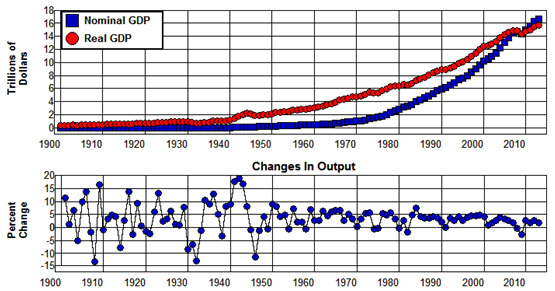
Nominal GDP and Real GDP measured in 2009 prices are plotted in Figure 1.4 from 1901 through 2013 using data from the Historical Statistics of the U.S. (Ca9, Ca10) for the years 1901 through 1928 and from the Bureau of Economic Analysis (1.1.5 1.1.6) for the years 1929 through 2010. Nominal GDP and Real GDP in Figure 1.4 are, of course, the same in 2009 since that is the base year—the year from which the prices used to measure the value of the output produced in all of the years were obtained.
Figure 1.4: Nominal and Real GDP (Prices=2009), 1901-2-13.
Source: Bureau of Economic Analysis. (1.1.5 1.1.6) Historical Statistics of the U.S. (Ca9, Ca10)
The values of Nominal GDP are below those of Real GDP in the years preceding 2009 in Figure 1.4 because prices in those years were, on average, lower than they were in 2009. As a result, the value of Nominal GDP measured in current prices—that is, in prices that existed at the time—in those years underestimate the differences in the total quantity of output produced relative to that produced in 2009. Similarly, the values of Nominal GDP are above Real GDP in the years following 2009 because prices in those years were, on average, higher than they were in 2009. As a result, the value of Nominal GDP in those years overestimate the differences in total quantity of output produced relative to that produced in 2009.
The year to year percentage changes in Real GDP (Changes in Output) are also plotted in Figure 1.4. These rates of change give us a measure of the rates as which aggregate (i.e., total output) output changes from year to year.
Finally, it should be noted that what we are doing here is adding apples and oranges, which everybody knows, you can't do. But, of course, you can add apples and oranges if you have a common unit of measurement, such as ponds or bushels. It is important to remember, however, that when you do this you don't end up with either apples or oranges, but, rather, ponds or bushels of fruit, and the sum tells us nothing at all about the kind of fruit that is included in the result. In measuring the total output produced within the economy, the common unit of measurement is the monetary unit, dollars, and the result of summing the various outputs of goods and services produced as measured in dollars is the total value of output produce—the real value if prices are held constant over time or the current or nominal value if the prices that are current at the time are used. In either case, the sum tells us nothing at all about the composition of the total or how the composition changes over time. This apples and oranges problem is intrinsic in all aggregate measures (measures arrived at by adding to obtain a total) of disparate economic variables.
Measuring Prices
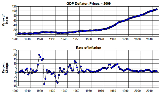
Since the difference between the value of nominal GDP and real GDP in each year is caused by the differences between current year prices and the prices that existed in the base year (2009 in Figure 1.4), if we divide nominal GDP by real GDP and multiply by 100 the result is a price index that expresses the weighted average (weighted by current year quantities produced) of current year prices to base year prices as a percent of base year prices. This index is called the Implicit GDP Deflator. A measure of the rate of inflation that includes all goods and services that are produced within the economy can be obtained from this index by calculating its year to year percentage changes.
The Implicit GDP Deflator in 2009 prices is plotted from 1900 through 2013 in Figure 1.5 using the GDP deflator implicit in the Historical Statistics of the U.S. (Ca10) for the years 1900 through 1928 and in the series published by the Bureau of Economic Analysis (1.1.5) for the years 1929 through 2013. The year to year percentage changes in this index that give the rate of inflation—that is, the rate of change in the average price as measured by the index—for each year is also plotted in this figure.
Figure 1.5: Inflation and GDP Deflator, 1900-2013.
Source: Bureau of Economic Analysis. (1.1.5) Historical Statistics of the U.S. (Ca10)
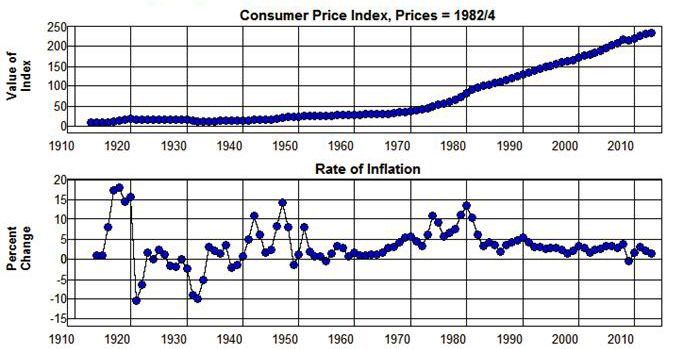
While the Implicit GDP Deflator provides a measure of the average price level of all goods and services produced in the economic system, the Consumer Price Index (CPI) provides a measure of the average price level of those goods and services that consumers purchase. It is constructed by surveying consumers to determine how they spend their incomes and creating a representative market basket that contains goods and services in proportion to the averages of the goods and services purchased by the consumers surveyed. Since the quantities in this market basket are fixed, and value of this market basket changes as prices change over time, if we divide the value of the market basket in each year by the value in some base year and multiply by 100 the result is an index that expresses the weighted average (weighted by the quantities in the representative market basket) of current year prices to base year prices as a percent of base year prices. A measure of the rate of inflation as it affects consumers can be obtained from this index by calculating its year to year percentage changes.
The Consumer Price Index (which uses the average value of the market basket for the period from1982 through 1984 for the base year) is plotted from 1913 through 2013 in Figure 1.6. The year to year percentage changes in this index are also plotted in this figure.
Figure 1.6: Inflation and Consumer Price Index, 1900-2013.
Source: Bureau of Labor Statistics.
Output, Productivity, and Employment
We can use real GDP as a measure of the output of goods and services produced in the economy, and by taking the year to year percentage change in this measure we can calculate the rate at which total output increases or decreases in each year. These rates are plotted in the bottom graph in Figure 1.4. They are important because the level of employment over time depends, in part, on the quantity of output produced. In general, an increase in the quantity of output produced is associated with an increase in employment and a decrease in the quantity of output produced is associated with a decrease in employment. However, the level of employment not only depends on the quantity of output produced, it also depends on the way in which output is produced.
The reason is that the amounts and kinds of tools and equipment and the ways things are done tend to increase and improve over time. These increases in the capital stock and improvements in technology (ways of doing things) tend to increase the productivity of labor over time which means they increase the amount of output a given number of workers can produce during a given amount of time. As a result, in order to maintain a given level of employment, real GDP must increase over time at the rate labor productivity increases. By the same token, in order to increase the level of employment, real GDP must increase at a rate that is greater than the rate at which labor productivity increases.
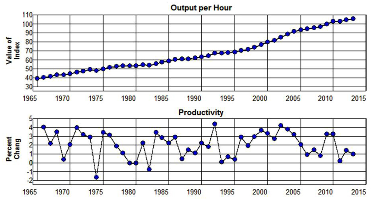
The Bureau of Labor Statistics’ productivity index of output per hour is plotted in Figure 1.7 from 1965 through 2013 along with the percentage changes in this index. The percentage changes in this index give the year to year rates at which labor productivity changed during each year.
Figure 1.7: Output and Productivity, 1965-2013.
Source: Economic Report of the President, 2014. (B49PDF|XLS)
From 1965 through 2013 this index increased from 39.4 to 106.2 which implies an effective annual rate of increase equal to 2.1% per year. This means that real GDP had to increase, on average, by 2.1% per year over the previous 48 years just to maintain the level of employment that existed in 1965. It also means that during those 48 years it was necessary for output to grow, on average, by 2.1% plus the rate at which the labor force grew in order to keep the labor force fully employed.