Summary
George H. Blackford © 2009, last updated 5/1/2014
Part I: Conservative Economic Policies
Part I examines how changes in economic policy over the past forty years have affected the economic system and explains how these policy changes have affected the way in which our economic system functions.
Chapter 1: Income, Fraud, Corruption, and Efficiency discusses the way in which deregulation and the change in attitude toward regulating economic behavior has led to a rise in fraud and corruption within our economic and political systems, and how this increase in fraud and corruption has, in turn, led to a loss in economic efficiency through the creation of speculative bubbles and an inequitable distribution of income derived from speculative rather than productive endeavors.
Chapter 2: International Finance and Trade discusses how deregulation in the area of international finance has led to international financial crises that have necessitated government bailouts of our financial institutions to keep them from failing. The way in which this change in policy has led to an overvalued dollar that has wrought havoc with the American economy as it devastated our manufacturing industries and transformed the United States from the largest creditor nation in the world to the largest debtor nation in the world is also discussed. The Appendix at the end of this chapter provides a primer on the way in which international exchange rates are determined and how these rates affect economic interactions between countries.
Chapter 3: Mass Production, Income, Exports, and Debt examines the relationship between mass-production technology, the distribution of income, exports, and debt within the economic system. It is argued that in order to be economically viable, mass production techniques require mass markets—that is, markets with large numbers of people who have purchasing power—otherwise, the mass quantities of goods and services that can be produced via mass-production techniques cannot be sold. The viability of mass markets within a society, in turn, depends on the distribution of income in that the distribution of income limits the extent to which domestic mass markets can be sustained without an increase in debt relative to income: The less concentrated the distribution of income, the larger the domestic mass market that can be sustained; the more concentrated the distribution of income, the smaller the domestic mass markets that can be sustained.
It is also argued that, in a mass production economy, the mass markets needed to obtain full employment can only be maintained in the face of an increasing concentration of income if there is an increase in debt relative to income. It is further argued that the process by which debt must be increased in this situation is unsustainable. As debt increases relative to income the strain on the financial system must grow, and, eventually, a financial crisis must result as the ability to service the growing debt falters. Hence, the financial crisis of 1929-1933 following the increase in debt and the concentration of income in the 1920s, the savings and loan crisis of 1987-1991 following the increase in debt and the concentration of income in the 1980s, and the current financial crisis following the increase in debt and the concentration of income in the 2000s.
Chapter 4: Going into Debt examines the relationship between the deregulation of our financial system and the rise of domestic debt from 1970 through 2010. The way in which financial institutions create debt through the process of financial intermediation is explained, and it is argued that there are powerful incentive within the financial system that lead financial institutions to fund speculative bubbles that increase debt beyond any possibility of repayment. When this occurs a financial crisis that brings down the economic system is inevitable. It is further argued that not only is this what happened during the housing bubble in the 2000s, it is also what happened during the real estate and stock-market bubbles of the 1920s, and the parallels between the between the 2000s and the 1920s are examined.
Part II: Financial Instability and the Crash of 2008
Part II explains how our financial system works and how the changes in economic policy that have occurred over the past forty years led to the economic catastrophe we are in the midst of today.
Chapter 5: Nineteenth Century Financial Crises gives a brief history of our financial system as it evolved during the nineteenth century. The way in which financial institutions—specifically, banks but any financial institution that finances long-term assets through short-term debt must be included here—differ from other businesses is examined.
The fundamental liquidity and solvency problems that are unique to banks are explained along with the way in which increasing leverage within the financial system leads to financial crises that cause economic instability. The fundamental mechanism by which banks create debt—namely, by virtue of the fact that banks are able to increase the amount of money they can borrow from the non-bank public by increasing the amount of money they lend to the non-bank public—is explained in this chapter.
The implications of the fundamental problems endemic in the banking system with regard to economic instability are examined as well as the failings of the nineteenth century banking systems that led to financial crises.
Chapter 6: The Federal Reserve and Financial Regulation explains the way in which our modern financial system is structured by the Federal Reserve. How the Federal Reserve determines the amount of currency that is available to the economic system is explained as well as how the interaction between the banking system and the non-bank public—given the amount of currency that is made available by the Federal Reserve—determines the amount of debt created by the banking system as the banking system increases the amount it can borrow by increasing the amount it lends.
The way in which the Crash of 1929 and the Great Depression of the 1930s led to a change in attitude toward the nineteenth century ideological dictates of free-market capitalism is also examined in this chapter. It is argued that the resulting change from an ideological to a pragmatic view of the economic system led to the creation of a comprehensive system of financial regulation in the 1930s through the 1960s that served our country well until we began to dismantled this system in the 1970s.
Chapter 7: Rise of the Shadow Banking System examines the process by which the pragmatic system of financial regulation created in the wake of the Great Depression was dismantled as the failed, nineteenth-century ideology of free-market capitalism began to gain favor again among policy makers in the 1970s.
The basics of financial markets and the nature of financial instruments are explained along with the changes in the financial system that came about through the creation of markets for collateralized debt instruments. It is shown how the change in attitude toward regulation, combined with the creation of markets for collateralized debt instruments, led to the rise of financial institutions—shadow banks—that operated outside the purview of the financial regulatory system and yet operated like banks in that they held long-term assets financed by short-term debt.
The way in which the shadow banks pose all of the treats to economic stability that an unregulated banking system poses is examined, and it is argued that since the shadow banks were allowed to operate outside the purview of the regulatory system, there was nothing to keep them from reverting to the kinds of behaviors that led to the kinds of crisis we experienced during the era of unregulated finance that culminated in the Crash of 1929 and drove us into the Great Depression of the 1930s.
Chapter 8: LTCM and the Panic on 1998 examines the first major financial crisis caused by a shadow bank: the worldwide panic that resulted from the near failure of a single hedge fund, Long-Term Capital Management (LTCM), in 1998.
It is shown that all of the problems endemic in the failure to regulate the shadow banking system—problems that subsequently led to the financial crisis we are in the midst of today—were acknowledged in the government reports on this crisis submitted by the President's Working Group and by the General Accounting Office.
It is further argued that ideological blindness on the part of policy makers in the Clinton administration and the Republican congress at the time made it impossible for those in charge of our government to even see the extent of the threat these problems posed let alone to follow the recommendations of the General Accounting Office and bring shadow banks under the purview of the regulatory system.
Chapter 9: Securitization, Derivatives, and Leverage explains the basics of the securitization process, the nature of financial derivatives, and the way in which financial derivatives increase leverage and, hence, risk within the financial system.
How Mortgage Backed Securities (MBSs) come into being is also explained in this chapter along with Collateralized Debt Obligations (CDOs), Credit Default Swaps, synthetic CDOs, and options and futures contracts.
The risks involved in trading financial derivative in over-the-counter markets as opposed to trading these kinds of financial instruments on exchanges with the protections provided by a clearinghouse are explained as well, and the reasons why the failure to regulate the markets for financial derivatives had such devastating consequences when the crisis began in 2007 are examined.
Chapter 10: The Crash of 2008 chronicles the events that led up to the Crash of 2008 and the way in which we dealt with the economic catastrophe that followed. It is argued that because of the extent to which debt was allowed to accumulate, and the extent to which the unregulated markets for over-the-counter derivatives were able to increase risk in the financial system, the financial situation we faced in 2008 was far worse than anything we faced in 1929.
It is further argued that there are but three threads by which the economy is hanging today that have made it possible for us to avoid, so far at least, the disastrous consequences that followed the Crash of 1929, and that these three threads are there only because of the size of our federal government. These three threads are 1) the heroic actions of the Federal Reserve in keeping the world's financial system from collapsing, 2) the size and stability of federal government expenditures that placed a break on the downward spiral of income and output that was initiated by the crash in 2008, and 3) the existence of our social-insurance programs that have mitigated the kind of human misery and suffering that, in the absence of these kinds of programs, inevitably accompany the kind of economic catastrophe we are in the midst of today.
Finally, it is argued that the free-market ideologues—whose mantra of lower taxes, less government, and deregulation brought on the economic crisis we are in the midst of today—are doing everything they can to cut the three threads by which our economic system is hanging, and in this Alice-in-Wonderland world in which we live there is every reason to believe they are going to do this if and when they regain control of the federal government.
Part III: The Federal Budget
Part III examines the history of the national debt, the federal budget, and our social-insurance programs in an attempt to sort through the sophistry endemic in the debate surrounding these entities. All of the data in these chapters are taken from the official statistics published in the Office of Management and Budget's Historical Tables or from other official government documents.
Chapter 11: History of the National Debt begins by explaining a number of definitions and relationships—such as definitions of gross and net national debt and the relationship between the national debt and surpluses and deficits in the federal budget—that are required to understand what the national debt is and where it comes from. The importance of measuring the national debt relative to some other variable in the economic system, such as GDP, is explained.
The history of the national debt is examined for the 83 years between 1929 and 2012. The basic conclusions that result are that the primary sources of the national debt are 1) increases in defense expenditures associated with war, 2) economic downturns associated with recessions and depressions, and 3) cutting taxes in the face of rising government expenditures. These conclusions are reinforced when we look at the history of the federal budget in the next chapter.
A number of technical issues surrounding the construction of aggregate measures of economic activity—such as measures of total output, the average price level, and the level of productivity in the economy—are explained in the appendix at the end of this chapter.
Chapter 12: History of the Federal Budget examines the history of the federal budget from the perspective of how our country has changed since 1929. All of the major categories of the federal budget are plotted in this chapter from 1940 through 2012.
It is argued that the loss of faith in free-market capitalism brought on by the Great Depression and our international interventionist policies brought on by World War II and the ensuing Cold War had profound effects on the American psyche that led to dramatic changes in the federal budget following 1929. In looking at the history of the budget we find that these factors led to a dramatic increase in the size of the budget relative to the economy in the 1930s through the 1950s, and that this increase was dominated in the 1940s by an increase in defense expenditures. We also find that while the size of the federal budget relative to the economy has been relatively constant since the 1960s, the composition of the budget has changed dramatically. The most dramatic change has been the decrease in the fraction of the budget that is devoted to defense and the increase in the fraction that is devoted to Human Resources—that is, devoted to the social-insurance programs that came out of Roosevelt's New Deal, the most important of which are Social Security and Medicare.
The primary mechanisms by which the increase in the Human Resources component of the budget has been financed over the past 60 years is seen to have been a decrease in expenditures on national defense and an increase payroll taxes as a percent of GDP. This decrease in national defense and increase in payroll taxes was used to finance a reduction of all other taxes collected by the federal government as well. The reduction of taxes on corporations has been especially dramatic in this regard.
Finally, it is argued that if we are to have less government the place we have to cut the budget is in the Human Resources portion of the budget and possibly defense since virtually everything else has been cut to the bone since 1980.
Chapter 13: Human Resources and Social-Insurance examines the portion of the federal budget devoted to the social-insurance programs (Human Recourses) that have grown out of Roosevelt's New Deal. This category of the budget has gone from 33.4% of the budget and 4.6% of GDP in 1950 to 64.4% of the budget and 12.7% of GDP in 2007. The great bulk of the expenditures in this category fund our social-insurance programs.
We find that Human Resources is dominated by federal healthcare and retirement programs and that Medicare, Medicaid, and Social Security dominate these programs. Healthcare and retirement went from 0.0% and 5% of the budget in 1940 to 25% and 26% of the budget in 2007, respectively. All other categories of Human Resources were less than 5% of the budget during the entire period. In terms of GDP, healthcare and retirement grew to 4.9% and 5.2% of the economy by 2007 while none of the other categories in Human Resources exceeded 1% of the economy during that period save unemployment compensation which hit 1.1% of GDP in 1976 following the 1973-1975 recession.
When we examine the data we find that 71% of the increase in the total costs of Human Resources programs since 1965 can be attributed to the increase in the cost of healthcare, 21% to the increase in the cost of federal retirement programs, less than 6% by the increase in the cost of federal non-healthcare, public assistance programs, and less than 3% by the increases in the cost of all other Human Resource programs combined.
Chapter 14: Welfare, Tax Expenditures, and Redistribution examines the welfare programs in the federal budget, that is, those programs the benefits of which are available to aid the poor and are specifically designed to redistribute income from those who are better off to those who are less fortunate.
We find that total welfare expenditures grew gradually from 1952 through1967 and then increased dramatically from 4.3% of the budget and 0.85% of GDP in 1967 to 16.3% of the budget and 3.2% of GDP in 2007. When we break these expenditures down into cash and non-cash benefits we find that expenditures on cash-benefit welfare programs relative to the economy and federal budget in 2007 was essentially the same as it was in 1965, less than 5% of the budget. We also find that while virtually all of the cash-benefit welfare payments went to people who were not employed in 1965, fully half of the cash-payment welfare expenditures went to the working poor in 2007, rather than to recipients who were not employed.
We also find that expenditures on non-cash assistance programs represented 73% of welfare expenditures in 2007 and only 27% of the welfare expenditures were cash benefit programs. At the same time, we find that the Medicaid program amounted to 7.0% of the budget in 2007 and, thus, accounted for 42% of all welfare expenditures in 2007 and 56% of all expenditures on non-cash assistance programs. None of the other welfare programs exceeded 2% of the budget in 2007 or 0.4% of our gross income. The single most important factor in driving up the cost of welfare since 1967 is to be found in the Medicaid program.
In addition to welfare expenditures, there were over 200 provisions in the federal tax code in 2007 that had the effect of redistributing income within our society. These provisions are referred to as tax expenditures, and since the benefits of tax expenditures are guaranteed by law to all who qualify for them, they are, in fact, entitlement programs.
In examining the various categories of tax expenditure entitlements in the federal budget we find that the extent to which tax expenditures redistribute income from the general tax payer to upper income groups far exceeds the extent to which welfare programs redistribute income from the general tax payer to lower income groups.
Part IV: Coming to Grips with Reality
Part IV examines the major economic problems with which we are faced today, the way in which we should deal with these problems, and the role played by ideology in creating these problems and in preventing solutions to these problems.
Chapter 15: Federal Versus Non-Federal Debt examines the fundamental difference between federal debt and non-federal debt and the lessons that should have been learned from the 1930s with regard to the importance of this difference as it relates to the stability of the economic system. It is argued that the most serious problem we face today is our non-federal debt, not our federal debt, and that it was the attempt to follow conservative fiscal and monetary policies from 1929 through 1933 that drove us into the debts of the Great Depression. It is also argued that the way in which our debt problem was solved during the 1930s and 1940s was by increasing economic growth, and the way the economic growth that solved our debt problem and took us out of the Great Depression was through a massive increase in government expenditures that was accompanied by dramatic increases in taxes.
Finally, is argued that none of the lessons that should have been learned from our experiences in the 1930s through the 1970s with regard to the federal debt have been learned by the free-market ideologues whose only vision for the future is lower taxes, less government, deregulation, and paying off the national debt. It is further argued that one of the lessons that should have been learned—namely, the need for higher taxes in this situation—has not been learned even by most of those who have learned the other lessons that should have been learned from our experiences of the 1930s through the 1970s.
Chapter 16: Managing the Federal Budget examines the fiscal problems we face. It is argued that if the government is to be made fiscally sound we must provide the government services that the people demand, and then collect the taxes necessary to pay for these services. It is further argued that this could be done quite easily by 1) rescinding the 2001-2003 Bush tax cuts, 2) eliminating unwarranted tax deductions and credits, 3) increasing the top marginal tax rates, and 4) increasing taxes on corporations.
It is also argued that if those who benefit the most from our economic system do not pay back in taxes enough to rebuild the public infrastructure and social capital that is consumed in the process of reaping the benefits they gained from our economic system, there is little hope for the future. It is further argued that this does not mean just the top one or two percent of the income distribution must pay back. It means that everyone who is capable of making a contribution toward this end must do their part. If this is not done we will consume the public resources that were left for us by previous generations, and in failing to replenish those resources, we will limit the economic possibilities for future generations.
Chapter 17: Social Security, Healthcare, and Taxes looks at the problems created by the baby boomers retiring with regard to Social Security, Medicare, and the federal budget.
The Moment of Truth report written by Erskine Bowles and Alan Simpson is examined in detail in this chapter and is found wanting. It is argued that there are many ways to deal with the relatively minor problems posed by the baby boomers retiring when it comes to Social Security that do not involve the drastic changes in Social Security called for by Bowles and Simpson. At the same time, it is argued that containing the cost of Medicare is a serious problem and that the engine that drives up cost in the Medicare program is to be found in the private healthcare system, not in Medicare itself.It is argued that t
he most obvious, simplest, most efficient, and most cost effective way to deal with this problem would be to extend the Medicare program to the entire population, thereby, providing a mechanism by which costs in the entire system can be controlled. It is further argued that if we are to preserve Social Security and Medicare and, at the same time, provide all of the other government programs and services demanded by the American people in a fiscally responsible way, we must raise taxes.Chapter 18: Ideology Versus Reality examines the extent to which free-market ideologues fail to perceive the real world as it actually is and the consequences to society that result from their failure to come to grips with reality. It is argued that this ideological view is based on a straw-man caricature of government that completely ignores all of the essential functions that government performs in our daily lives and without which civilized society is impossible, and the academic model that explains how, and under what circumstances a free-market economy is supposed to work not only completely ignores the role of government in our economic and social lives, but the assumptions on which the logical consistency of this model depends are impossible to achieve in the real world.
Chapter 19: Beyond the Current Crisis goes beyond the current economic disaster caused by deregulating the world’s financial system. It is argued that globalization, combined with technological improvements in transportation and communication over the past thirty years have led to incredible growth in productivity and output throughout the world. Unfortunately, this growth is derived from the same failed, nineteenth-century ideological paradigm of free-market capitalism that led to the deregulation of our financial system.
This paradigm is terribly flawed in its failure to understand the necessity to regulate pollution and to preserve our natural resources. If we value the kind of world we leave to our children and grandchildren we cannot sit back and hope for the best as unregulated markets squander our natural resources and pollute our planet. It is argued that the problems posed by population growth, the worldwide drive to industrialize, and the finite nature of our natural resources cannot be solved by markets alone. They can only be solved through the international cooperation of governments.
Autobiographical Information and Acknowledgements provides some autobiographical information and attempts to acknowledge the contributions others have made to whatever accomplishment I may have achieved in life.
Selective Bibliography lists a number of books that have contributed to my understanding of how the world works.
![]()
Chapter 1: Income, Fraud, Corruption, and Efficiency
George H. Blackford © 2009, last updated 5/1/2014
![]()
There’s class
warfare, all right, but it’s my class, the rich class,
that’s making war, and we’re winning.
Warren E. Buffett
Changes in the economic landscape over the forty years leading up to the 2007 financial crisis are astounding. This is particularly true when it comes to changes in the tax code. The maximum marginal income tax was reduced from 70% to 35%, the maximum capital gains tax from 28% to 15.7%, the maximum corporate profits tax from 50% to 34%, the maximum tax on dividends from 70% to 15%, and the maximum marginal estate tax from 70% to 35%. At the same time, payroll taxes were increased as were taxes on cigarettes, alcohol, and other sales and excise taxes as government fees and fines and the tuition at public colleges and universities were increased as well. All of these changes have made our system of government finance more regressive—that is, they increased the proportion of income taken by the government from low and middle-income groups relative to the proportion taken from upper-income groups. (PCCW)
Changes in the area of market regulation have been particularly dramatic as well. Much of our regulatory system had been dismantled, either through legislative changes, deliberate under funding of the regulatory agencies, or through the appointment of individuals to head these agencies who did not believe in regulating markets and were willing to restrict the enforcement of existing regulations. (Frank Kuttner Amy NYT Bair)
A third area of economic policy in which there have been profound changes is in the area of international finance and trade. Of particular importance was the abandonment in 1973 of the managed international exchange system set up by the Bretton Woods Agreement in 1944 and replacing it with what became known as the Washington Consensus which championed unrestricted international finance and trade. This eventually led to innumerable bilateral trade agreements negotiated with China since Nixon's historic visit in 1972, the North American Free Trade Agreement in 1994, and our joining the World Trade Organization in 1995. (Mavroudeas Stiglitz Galbraith Reinhart Philips Morris Eichengreen Rodrik)
All of these changes were championed in the name of economic efficiency and have, in fact, made it possible for countless individuals to amass huge amounts of wealth over the past forty years. What’s wrong with that? Haven’t we all benefited from the generation of all that wealth? Well, not exactly.
Changes in the Distribution of Income
It is instructive to look at how the distribution of income has changed since the onset of the changes in economic policy mentioned above.
Bottom 90%
Figure 1.1 shows the average real income, both including and excluding capital gains, measured in 2012 prices, of all families in the bottom 90% of the income distribution in the United States from 1917 through 2012. In 2012 this group consisted of 145 million families that received an income (including capital gains) of $113,820 or less. The average income for this group was $30,997 in 2012.
Source: The World Top Incomes Database.
It is clear from Figure 1.1 that the 90% of the families at the bottom of the income distribution did not benefit at all from the increase in income that occurred from 1973 through 2012. While the average real income of this group rose dramatically from 1933 through 1973, increasing by a factor of 5, it trended downward from 1973 through the 1980s and didn't start to trend upward again until 1993. This upward trend was short lived, however, as the real income for the lower 90% began to decrease again after 2000.
The average real income of the bottom 90% of the income distribution actually fell by 13% during the 39 year period from 1973 through 2012. This 13% decrease provides a stark contrast to the 368% increase in real income this group experienced in the 39-year period that proceeded 1973. In absolute terms, average real income increased by $27,985 from 1934 through 1973 and fell by $4,587 from 1973 through 2012. The $30,997 average income the bottom 90% of the income distribution received in 2012 was actually less than the $31,006 average this income group received 46 years ago in 1966.
The fall in average real income from 1973 through 2012 received by the bottom 90% of the income distribution is particularly stark in light of the 104% increase in productivity that took place in the economy during this period. None of the benefits of this increase in productivity went to the bottom 90% of the income distribution. (Saez Gordon Sum)
Top 90-99%
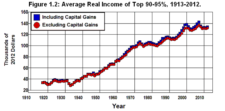
As is indicated in Figure 1.2, the situation was somewhat better for families in the top 90 to 95% of the income distribution. In 2012, this group consisted of the 8.0 million families that received an income between $113,820 and $161,438. The 2012 average income for this group was $133,530.
Source: The World Top Incomes Database.
Like the bottom 90%, the average real income of this group rose dramatically from 1933 through 1973, increasing by a factor of 3.75. After 1973, its average income leveled off but began an upward trend in 1982 that peaked in 2000 and again in 2007. It then receded somewhat by 2012. While the average real income of this top 90 to 95% of the population did increase by 25% from 1973 through 2012, this increase for that 39-year period was a mere fraction of the 251% increase this group experienced during the 39 years that proceeded 1973 and a third ($26,704) of the $76,375 increase this group received in absolute terms during this 39-year period.
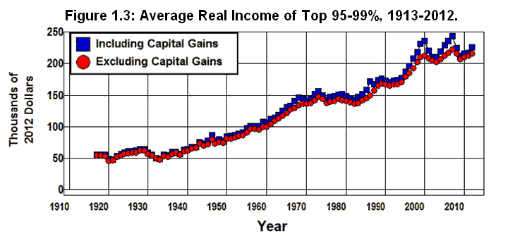
The pattern in Figure 1.2 repeats itself in Figure 1.3 for the next 4% of the income distribution. In 2012, this group consisted of 6.4 million families that received between $161,438 and $393,941, and the 2012 average income for this group was $226,405. The 44% increase in real income for this group for the 39-year period following 1973 was, again, far less than the 187% increase for this group during the 39-year period before 1973 and only 68% ($69,669) of the $102,127 increase they had received in absolute terms during this period.
Source: The World Top Incomes Database.
Top 1%
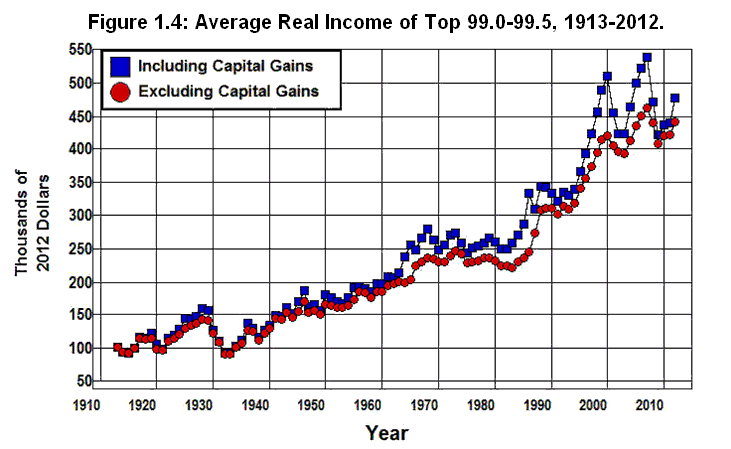
It's not until we get to the top 1% of the income distribution that this pattern changes, though not everyone in this group benefited equally. Figure 1.4 shows the average income of the top 99.0 to 99.5% of the income distribution. In 2012, this group consisted of 803,405 families that received between $393,941 and $611,805 with an average income of $477,738.
Source: The World Top Incomes Database.
The average real income of this group increased by 74% during the 39-year period from 1973 through 2012, a significant improvement over lower-income groups. Even though this is less than half of the 165% increase this group received in the 40-year period preceding 1973, the $203,097 increase in real income that took place from 1973 through 2012 is at least greater than the $171,155 increase in real income that this group received from 1934 through 1973.
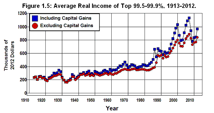
It's not until we get to the top 1/2 of the top 1%, however, that we come to the first income group that unambiguously benefited from the changes in tax, deregulatory, and international policies wrought by the policy changes that have taken place during the past forty years. Figure 1.5 through Figure 1.7 break down the top half of the top1% of the income distribution into three Groups:
Figure 1.5 shows the average income of the top 99.5 to 99.9% of the income distribution. In 2012, this group consisted of 642,724 families that received incomes between $611,805 and $1,906,047 with an average income of $969,544.
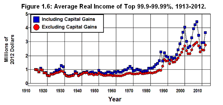
Figure 1.6 shows the average income of the top 99.9 to 99.99% of the income distribution. In 2012, this group consisted of 144,613 families that received incomes between $1,906,047 and $10,256,235 with an average income of $3,661,347.
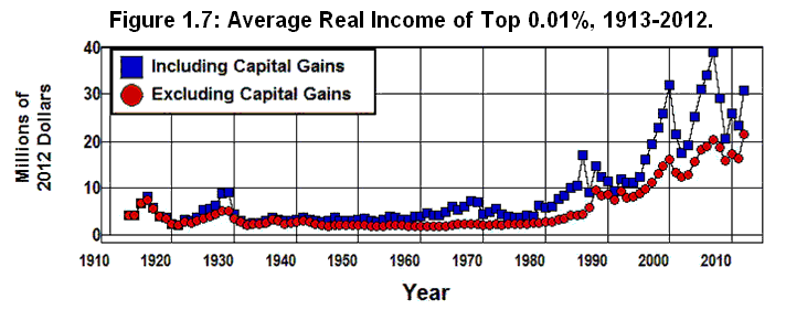
Figure 1.7 shows the average income of the top 0.01% of the income distribution. In 2012, this group consisted of 16,068 families with incomes equal to or above $10,256,235 with an average income of $30,785,699.
Source: The World Top Incomes Database.
Here are the true benefactors of the changes in tax, deregulation, and international trade policies over the past forty years. While the average real income of the bottom 90% of the population fell from $36 thousand a year in 1973 to $31 thousand a year in 2012, the average real income of the top 0.5% of the population more than tripled:
For the top 99.5-99.9% it went from $426 thousand to $970 thousand a year, a $544 thousand increase compared to a $231 thousand increase from 1934 through 1973.
For the top 99.9-99.99% it went from $971 thousand to $3.7 million a year, a $2.7 million increase compared to a $402 thousand increase from 1934 through 1973.
And for the top .01% it went from $4.5 million to $30.8 million a year, a $26.3 million increase compared to a $1.9 million increase from 1934 through 1973, all measured in 2012 dollars.
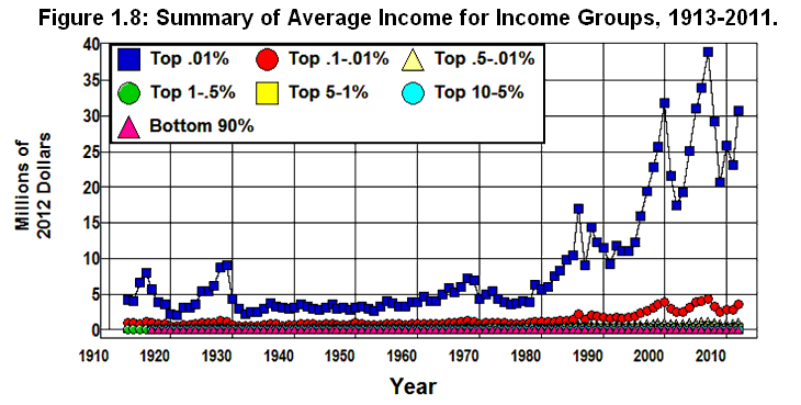
The relative magnitudes of the numbers involved can be seen in Figure 1.8 which plots the average incomes (including capital gains) of the various income groups from 1913 through 2011 on the same scale.
Source: The World Top Incomes Database.
Summary
This is what the changes in economic policy in the name of free-market capitalism and economic efficiency over the past forty years have led to, namely, a huge windfall for the upper 0.5% of the income distribution, a net loss for the bottom 90% of the income distribution, and relatively little if anything for the 90-99.5% of the income distribution in between. (Piketty Saez Gordon Sum) What's more, the situation is even worse for those families at the bottom 90% of the income distribution than the above numbers indicate.
The average income of the bottom 90% would have fallen even further than the 13% indicated in Figure 1.1 were it not for the fact that the percentage of women who participate in the labor force has increased over 30% since 1973. This suggests that the number of two income families in the bottom 90 percent of the income distribution must have increased significantly during this period as mothers were forced to leave their children to the care of others and enter the labor force in order to maintain their family's standard of living.
When this is combined with a more highly regressive tax structure—higher payroll taxes, excise taxes, fines and fees, and higher tuition at public colleges and universities—it is clear that the 90% of the population at the bottom of the income distribution is significantly worse off today than it was forty years ago.
Deregulation and the Savings and Loans
The effects of changes in regulatory policy began to manifest themselves early in the1980s after the Depository Institutions Deregulation and Monetary Control Act of 1980 and Garn–St. Germain Depository Institutions Act were passed. These acts 1) lessened the capital and reserve requirements of banks, 2) provided mechanisms to assist failing banks rather than closing them down, 3) phased out interest rate ceilings on bank deposits, and 4) expanded the kinds of loans thrifts (savings and loans and savings banks) could make so as to allow them to become more like commercial banks. (FDIC) The purpose of these acts was to enhance the level of competition in the financial markets in order to improve the economic efficiency in these markets. This is not exactly how this grand experiment in deregulation worked out.
The early 1980s was a particularly ominous time to deregulate the savings and loans. At the end of the 1981 recession 10% of the savings and loans were insolvent on an accounting basis, and institutions that had no tangible equity at all controlled 35% of the industry's assets. (Black FDIC) These savings and loans—with their federally insured deposits—were allowed to compete on an equal footing with the rest of the financial system in spite of the fact that insolvent financial institutions have nothing to lose by rolling the dice and betting the farm on high stakes investments in trying to recoup their losses. After all, if they win they keep it all. If they lose, they just increase their insolvency, and since they were bankrupt to start with, they are no worse off than they were before. Their investors and taxpayers take the increased losses if they lose, not the owners and managers of the savings and loans. (Garcia)
What's more, the reduced regulation and supervision created innumerable opportunities to exploit the system through fraud. As a result, the character of the savings and loan industry changed after deregulation as a new breed of owners, such as Charles H. Keating and Hal Greenwood Jr., began to shift out of home mortgages and into commercial real estate loans, direct investments in real estate projects, junk bonds and other securities, and innumerable other risky areas where the potential for fraud abounds—areas they had been barred from entering since the 1930s as a result of the lessons learned from the 1920s. (FDIC Black Akerlof Stewart)
There was a virtual explosion in Acquisition, Development, and Construction (ADC) loans issued by savings and loans following deregulation whereby real estate developers were allowed to borrow money for a project with no interest or principal payments for three years. The savings and loans added huge fees to these loans, which they booked as income in the year the loans were made. The interest was also booked as income as it accrued over the three years of the loan even though no interest was paid. This led, through the magic of accounting, to huge paper profits out of which the owners and managers of the savings and loans paid themselves huge dividends, salaries, and bonuses in real cash even though no cash had been received for fees or interest owed.
What happened when the loans came due and the developers couldn't pay? No problem. The savings and loans just refinanced the loans, added more fees and interest to the principal, booked more paper fee and interest income, and paid themselves more dividends, salaries, and bonuses in real cash. And they were allowed to finance all of this through brokered deposits—federally insured certificates of deposit that were sold by brokerage firms, such as Merrill Lynch, to investors all over the country. The money from federally insured brokered deposits allowed the savings and loans to expand their deposit base, expand their ADC loans, finance innumerable other fraudulent schemes, increase their paper profits, and to come up with the real cash necessary to finance the huge payments of dividends, salaries, and bonuses that their managers and owners took out of these institutions. (Black Akerlof Stewart FDIC)
While this was going on, the inflow of credit into a number of regional commercial real estate markets that accompanied this expansion of savings and loan activity, mostly in the Southwest and Northeast, started speculative booms in these markets. As these bubbles developed, the fraudulently managed institutions began to threaten the honestly managed institutions—not just among the savings and loans but among the savings and commercial banks as well. Fraudulently managed savings and loans bid fiercely for brokered deposits as they bid up the rates paid on these deposits. This, in turn, increased costs in the entire financial system as the fraudulently managed savings and loans dug the hole deeper for everyone. Honestly managed institutions that were forced to, or were naively willing to invest in the booming commercial real estate markets made the situation worse.
ADC scams were not the only scams that followed in the wake of the deregulation of the early 1980s. Deregulation made it possible for Michael Milken and other corporate raiders of the 1980s to finance their leveraged buyouts and hostile takeovers by funneling the junk bonds they issued into captive savings and loans as they used the assets of the target companies as collateral for the junk bonds they issued. The proceeds from the sale of those bonds were then used not only to payoff the existing stockholders but to pay huge dividends and bonuses to the raiders themselves as the companies taken over were driven into bankruptcy along with the savings and loans that financed them.
As the speculative bubbles in the markets fueled by ADC scams burst and the companies taken over in junk bond scams began to go bankrupt toward the end of the 1980s and into the 1990s, the result was the first major financial crisis in the United States since the Great Depression. (FDIC) In the end, some 1,300 savings institutions failed, along with 1,600 banks. That amounted to almost a third of all savings institutions along with 10% of all banks in existence at the time. By comparison, only 243 banks failed between 1934 and 1980. In addition, some 300 fraudulently run savings and loans that were nothing more than Ponzi schemes failed at the peak of this disaster.
In the end, the corporate raiders and owners and managers of the savings and loans walked away with billions, and the tax payers took the losses. It costs the American taxpayer $130 billion to reimburse the depositors in these failed institutions. In addition, the resulting financial crisis was a precursor to the 1990-1991 recession. (Black FDIC Krugman Akerlof Stewart)
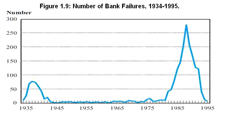
While the number of banks that failed during this crisis was only a third of the number that failed during the Great Depression, the extraordinary nature of the savings and loan crisis is indicated by the graph constructed by the FDIC that is displayed in Figure 1.9. This chart shows the number of FDIC insured commercial and savings banks that failed each year from 1934 through 1995. While it includes only the 1,600 FDIC insured institutions that failed and does not include the 1,300 failed savings and loans insured by the FSLIC, it clearly indicates the degree of stability in the system since the end of World War II through the 1970s before the era of deregulation began in earnest, and the degree to which deregulation in the 1980s destabilized the system.
Source: FDIC
The Rise of Predatory Finance and Corruption
While there was an attempt by Congress to reregulate the financial markets in the late 1980s and early 1990s, and taxes were raised somewhat during the late Bush I and early Clinton administrations, (TF TAP) the cat was out of the bag. The fortunes made by those who looted the savings and loans during the 1980s clearly demonstrated how lower tax rates on unearned and ultra high incomes combined with a lack of oversight on the part of government regulators made it possible for fortunes to be made by those willing to bend or ignore the law. Even though over a thousand individuals associated with the savings and loan debacle were convicted of felonies, most walked away with their fortunes intact. (Black Akerlof Stewart) This was the lesson learned by those at the top of the economic food chain, and this same lesson was drawn from the experiences in other industries as well.
Throughout the 1980s, fortunes were made through junk bond financing of hostile takeovers and leveraged buyouts that led to the dissolution of American companies, repression of wages, the looting of corporate pension funds and other assets, and the outsourcing of American jobs overseas and to Mexico. (Stewart Smith) Usury laws were repealed throughout the country, and credit card companies were allowed to charge exorbitant interest rates, exact unreasonable fees, and to manipulate payment dates and the dates at which payments were recorded to force customers to pay late charges even though they had mailed their payments on time. (PRIG) At the same time, credit card companies devised elaborate schemes to lure naive and financially unsophisticated customers deeper and deeper into debt. (Frontline MSN)
With so much money involved, the lack of government regulation allowed the entire fiduciary structure of our economic and political systems to become corrupted. Throughout the 1980s and 1990s stockholders lost control of corporations as the corporate governance structure broke down. Boards of directors became vassals of their CEOs, and management salaries and bonuses soared to astronomical levels. The major accounting firms found they could make more money advising corporations how to make paper profits in order to justify increases in management salaries and bonuses than they could by providing independent audits of companies' books for stockholders. Brokerage firms found they could make more money hyping worthless mutual funds and internet, energy, and telecom stocks than they could by providing sound investment advice to their clients. Investment banks found it more profitable to dissolve their partnerships, become corporations, and speculate for their own account with investors' money than to provide underwriting and advisory services to their clients. (Bogle Galbraith Stewart Baker Kuttner Phillips)
All of this involved huge conflicts of interest between corporation and mutual fund managers and the stockholders these managers are supposed to serve, accounting firms and the investing public the accounting firms are supposed to serve, brokerage firms and the investors the brokerage firms are supposed to serve, and investment banks and the businesses the investment bankers are supposed to serve. These conflicts of interest contributed directly to the Drexel Burnham Lambert, Charles Keating, Michael Milken, Ivan Boesky, and other insider trading, junk bond, and Savings and Loan frauds that were a direct cause of the junk bond, and commercial real estate bubbles of the 1980s, the bursting of which was a precursor to the 1990-1991 recession. They also contributed directly to the HomeStore/AOL, Enron, Global Crossing, and WorldCom frauds that were a direct cause of the dotcom and telecom bubbles of the 1990s, the bursting of which led to the 2001 recession.
In addition, throughout this entire period, antitrust laws were ignored as corporations were allowed to merge into mega institutions with overwhelming economic and political power. Laws against interstate banking were repealed in 1994, (IBBEA) and as the banking industry began to concentrate its power, key regulatory constraints on the financial system were removed in 1999 with the repeal of the Glass-Steagall prohibition against commercial bank holding companies becoming conglomerates that provide both commercial and investment banking services along with insurance and brokerage services. (FSMA) In 2000, the Commodity Futures Modernization Act which blocked attempts to regulate the derivatives markets was passed.
These changes made possible the accumulation of wealth in the 1980s, 1990s, and 2000s at levels that were heretofore unimaginable. Along with that wealth came unimaginable levels of economic and political power. And along with that power came a virtual collapse of integrity in our financial and political systems. In the wake of the dotcom and telecom bubbles bursting and the collapse of the HomeStore/AOL, Enron, Global Crossing, and WorldCom frauds, the mega banks and accounting firms that facilitated these frauds found they could make hundreds of billions of dollars by securitizing subprime mortgages. This discovery set in motion a set of forces that drove our economic system—along with that of the entire world—headlong into a catastrophe of epic proportions.
Securitization and the Crash of 2008
Securitizing subprime mortgages became so profitable that by the early 2000s there were not enough qualified subprime borrowers to meet the demands of the securitizers.[1.1] Rather than cut back their operations, predatory mortgage originators (such as Washington Mutual, Countrywide, IndyMac, New Century, Fremont Investment & Loan, and CitiFinancial) talked millions of naive people into applying for subprime mortgages by misrepresenting the nature of these mortgages. The most serious misrepresentation was to offer borrowers an adjustable rate, negative amortization mortgage with an unreasonably low teaser rate without explaining the effect on their monthly payment when the initial rate adjusted to the market rate. Using this and other ploys, borrowers who qualified for modest subprime mortgages at reasonable subprime rates, were talked into applying for exorbitant subprime mortgages at rates they could not afford. Even borrowers who qualified for modest prime rate mortgages at reasonable prime rates, were talked into applying for exorbitant subprime mortgages they could not afford. At the same time, borrowers not qualified for any kind of mortgage at all were approved for subprime mortgages. (Senate FCIC WSFC Spitzer)
Next, in order to sell these mortgages it was necessary for mortgage originators to obtain appraisals of the underlying properties consistent with the values of the mortgages being originated. To obtain these appraisals mortgage originators shopped around for appraisers who would write consistent appraisals and shunned appraisers who would not. This guaranteed rising incomes for appraisers that cooperated with the mortgage originators and falling incomes for those that did not. At the same time, some lenders setup in-house mortgage appraisal subsidiaries so as to guarantee the kinds of appraisals they wanted. The result was a systematic upward bias in real-estate appraisals, and the flow of funds into the real estate sector led to a systematic upward bias in housing prices. (FCIC WSFC)
As it became more difficult to find subprime borrowers, the securitizers turned to alt-A borrowers. At this point real-estate speculators got into the act. As housing prices rose, speculators discovered they could get alt-A mortgages with little or no money down and without any verification of the assets, income, or employment status they reported on the applications for these loans. These no-doc loans, as they were called in the beginning, were soon to become known as ninja loans—short for No Income, No Job, and no Asset loans—or just plain liar loans. As a result, a host of speculators took out alt-A mortgages knowing that if the prices of their properties increased they would profit greatly, and if the prices of their properties went down they could walk away from these mortgages with little or no loss to themselves. When such financing was combined with fraudulently obtained appraisals, many speculators were able to walk away from their loans with a profit without making a single payment on their mortgage. (T2P Senate FCIC WSFC)
Firms that securitize mortgages were the next link in the financial food chain that fed off the subprime and alt-A mortgages. In order for investment banks and other firms that securitized mortgages to sell the Mortgage Backed Securities (MBSs) at the highest possible price they had to receive the highest possible ratings from a bond rating agency. To accomplish this, the securitizers followed the lead of the mortgage originators to steer their business to bond rating agencies that gave them the highest ratings and away from those that gave them lower ratings. In this way the companies that securitized mortgages were able to get the three major bond rating agencies (Moody’s, Standard and Poor’s, and Fitch) to give triple-A ratings to mortgage backed securities even though the rating agencies had no creditable basis on which to rate these securities. (House FCIC WSFC)
From 2002 through 2007, literally millions of fraudulent obtained subprime and alt-A mortgages provided the collateral for trillions of dollars of Mortgage Backed Securities (MBSs) that were spread throughout the financial system of the entire world. (T2P FCIC WSFC) As these toxic MBSs spread around the world—as well as into banks, insurance companies, pension funds, money market funds, mutual funds, and institutional endowment funds at home—hundreds of billions of dollars were paid out in salaries, bonuses, and dividends to those who participated in the securitization process. Even the managers of the banks, insurance companies, and mutual and endowment funds that bought these toxic assets—and whose stock holders eventually suffered losses as a result—were paid billions of dollars as their paper profits grew along with the housing bubble.
Huge fortunes were amassed as this process grew beyond all bounds of reason, and as the fraud grew in the subprime and alt-A mortgage markets the officials in control of the federal government during the Bush II administration did nothing to stop it. When state or local authorities complained to the federal government about the predatory lending practices in their communities, not only did the Federal Reserve—which had the absolute authority under the Home Ownership and Equity Protection Act (HOEPA) to stop these practices (Natter WSFC)—do nothing to clamp down on the predatory practices in the mortgage market, the Bush II Justice Department actually went to court to keep state and local authorities from regulating this market. (Spitzer FCIC WSFC) As a result, no restraints were placed on the mortgage originators, securitizers, or bond rating agencies as the entire securitization process became corrupted.
The resulting housing bubble grew dramatically in the early 2000s, and as with all speculative bubbles, it was only a matter of time before it burst. By the time it did, $10 trillion worth of mortgages on residential properties with inflated prices were created that could not sustain their value. To make things worse, virtually all of the worst of the worst mortgages—the fraudulently obtained subprime and alt-A mortgages—were bundled into Mortgage Backed Securities and sold all over the world, and over half of the triple-A rated tranches of those MBSs ended up on the books of our own financial institutions—on the books of investment and commercial banks, money market funds, mutual funds, pension funds, and insurance companies throughout the country. (NYU)
As housing prices began to fall, the Mortgage Backed Securities that were created while housing prices were driven up to unsustainable levels lost their value and the ensuing panic drove all of the investment banks and most of the major commercial banks in our country into insolvency. To keep the financial system from collapsing and driving the economy into a depression comparable to that of the 1930s, the government had to step in and prop up the financial system with $700 billion in TARP funds. At the same time, the Federal Reserve was forced to increase reserve bank credit by over $1.5 trillion dollars in order to end the resulting run on the financial system. In the meantime, the unemployment rate hit 10%; trillions of dollars of wealth held by insurance companies, mutual funds, pension funds, and 401Ks evaporated, and the financial and international exchange systems of the entire world were destabilized as a worldwide economic crisis followed in the wake of this disaster. (Stiglitz NYU FCIC WSFC)
Speculative Bubbles and Economic Efficiency
The securitization of fraudulently obtained subprime and alt-A mortgages in the early to mid 2000s was, undoubtedly, the greatest fraud in history, one that sent shockwaves throughout the entire world. Those who bought homes during the housing bubble facilitated by this fraud, whose pension plans were invested in the toxic assets created as a result of this bubble, who had a stake in the endowment and mutual funds that invested in these assets, the small investors with 401Ks, those who depend on wages and salaries for their livelihood and found themselves unemployed as a result of the economic collapse caused by the bursting of the housing bubble, and those who lost their homes as a result of the collapsing housing market and the recession that followed were particularly hard hit by the economic catastrophe that followed in the wake of this disaster. At the same time, many, if not most of those who stood at the center of this fraud made fortunes. (FCIC WSFC)
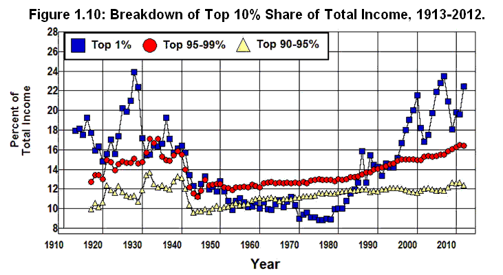
The same is true of the economic disasters that followed the hostile takeover/leverage buyout craze and the savings and loan fiasco of the 1980s and the dotcom and telecom bubbles of the late 1990s and early 2000s. Huge profits, bonuses, and windfall gains were generated as asset prices were bid up in the process of creating these speculative bubbles, and all of these bubbles were precursors to economic catastrophes. (Stewart FCIC WSFC) The extent to which this is so is shown in Figure 1.10through Figure 1.12.
Figure 1.10 provides a breakdown of the share of total income (including capital gains) that went to the top 10% of the income distribution from 1913 through 2010. This graph shows the relative stability of the share of total income of the top 90-99% of the income distribution since1945 compared to that of the top 1%. It also shows the volatility of the share of total income that went to the top 1% before 1945 and after 1980 compared to the relative stability of the share this group received in the period of restrictive financial regulation from 1945 to 1980. Of particular interest is the way in which the volatility of the top 1% is tied to speculative bubbles.
Source: The World Top Incomes Database.
The extent to which the top 1% of the income distribution benefited from these bubbles is clearly shown in Figure 1.10 by:
the 53% increase in income share this group received during the 1921-1926 real estate bubble and the 1926-1929 stock market bubble that led up to the Great Crash of 1929 and the Great Depression of the 1930s,
the 55% increase in income share this group received during the 1981-1988 junk bond, and commercial real estate bubbles of the 1980s that led up to savings and loan crisis and the 1990-1991 recession,
the 51% increase in income share this group received during the 1994-2000 dotcom and telecom bubbles that led up to the stock market crash of 2000 and the 2001 recession, and
the 39% increase in income share this group received during the 2002-2007 housing bubble that led up to the Great Crash of 2008 and the worldwide economic crisis we are in the midst of today.
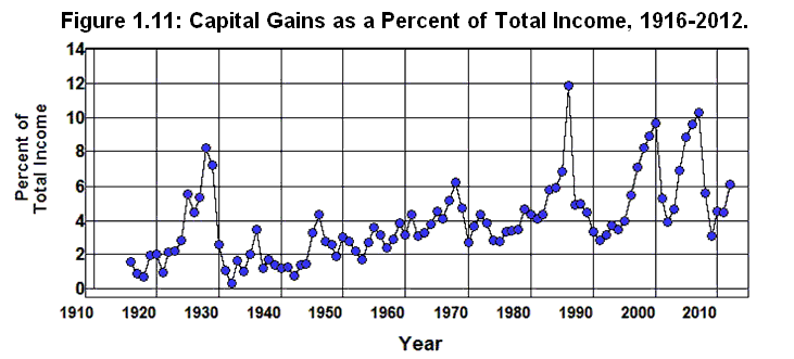
Similarly, Figure 1.11 shows the amount of income received in the form of capital gains as a percent of total income from 1916 through 2012. This figure displays a pattern similar to that in Figure 1.10 with relatively little volatility in the percent of total income received in the form of capital gains during the period of restrictive financial regulation from 1945 to 1980 compared to the preceding and following periods. While the 1986 spike in this graph conflates the effects of the anticipated 1987 increase in the capital gains tax with the effects of the stock market and commercial real estate bubbles of the 1980s, there were no capital gains tax increases in the 1920s, 1990s, or 2000s.
Source: The World Top Incomes Database.
The increase in capital gains by fully 6% of total income in the 1920s, 1990s, and 2000s depicted in Figure 1.11 clearly shows the effects of speculation on income during these eras that led to economic catastrophes as those who profited from these bubbles realized huge capital gains, and it is, perhaps, worth emphasizing here that these are realized capital gains. When the crash came there was someone or some institution on the other side of the sale that generated these realized capital gains that realized the loss including pension funds, insurance companies, 401ks, endowment funds, and taxpayers when depositors and financial institutions were bailed out.
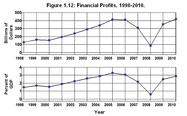
While Figure 1.10 and Figure 1.11 deal with family income, Figure 1.12 shows how the financial system fared through the housing bubble of the 2000s both in nominal terms and as a percent of GDP.
Source: Economic Report of the President, 2012 (B91PDF|XLS);
Bureau of Economic Analysis (1.2.5).Of particular interest in Figure 1.12 is the 163% increase in financial sector profits from 2000 through 2006 following passage of the Financial Services Modernization Act in 1999 and the Commodity Futures Modernization Act in 2000. These two acts, combined with the refusal by the Bush II administration and the Greenspan Federal Reserve to enforce what little financial regulation remained gave the non-depository financial institutions a free hand to do just about whatever they wanted to do in the world of finance. What they wanted to do was securitize millions of fraudulently obtained subprime and alt-A mortgages and sell those mortgages all over the world. In the process they accumulated over a trillion dollars in additional profits from 2001 through 2007 in excess of what they would have made if there had been no housing bubble and their profits had stayed at their 2000 level.
Deregulation of the financial markets was done in the name of economic efficiency, but the massive fortunes made in the process of creating the dotcom and housing bubbles had nothing to do with economic efficiency. Nor were there economic efficiencies gained in the fortunes made in the commercial real estate and junk bond bubbles created during the savings and loan fiasco or in the leverage buyout/hostile takeover craze of the 1980s or in the credit card predation that has grown in such immense proportions during the past thirty years.
These fortunes were amassed in the process of squandering our economic resources on a massive scale as companies were driven dangerously into debt through leveraged buyouts and hostile takeovers or in attempting to avoid such takeovers; funds were directed into sham internet companies, and resources were directed into the production of redundant telecom facilities and innumerable real estate projects that sat empty as the bubbles burst and millions of people lost their jobs, their homes, their pensions, their life savings, and their hopes and dreams for the future in the wake of the economic catastrophes that followed.
Economic efficiency means producing more with a given amount of resources toward the end of improving human well being. It’s not about transferring income and wealth from the bottom of the income distribution to the top. This transfer of income and wealth may seem efficient from the perspective of those at the top. It is clearly not efficient from the perspective of the vast majority of the population at the bottom. The suggestion that the policy changes that have occurred over the past forty years—policy changes that led to a collapse of the fiduciary structure of society, gave rise to massive frauds, generated massive rewards for those who perpetrated these frauds, and harmed the vast majority of the population to the benefit of the few—have somehow improved the economic efficiency of the American economy is absurd.
Over 8 million people had lost their jobs by 2010 as a result of the housing bubble bursting in 2006, and 4 million families lost their homes. In 2010, another 4.5 million families were seriously behind in their mortgage payment or in the process of foreclosure. “In the fall of 2010, 1 in every 11 outstanding residential mortgage loans in the United States was at least one payment past due but not yet in foreclosure.” Nationwide, 10.8 million families—22.5% of all families with mortgages—owed more on their mortgages in 2010 than their houses were worth. In Florida, Michigan, and Nevada more than 50% of all mortgages were underwater, and it is projected that by the time this crisis is over as many as 13 million families could lose their homes. (FCIC)
These numbers are the end result of the economic policy changes we have made over the past forty years, and there’s nothing efficient about them.
Endnote
[1.1] The basic mechanism by which securitization is accomplished, while complicated in practice, is fairly simple in principle:
First, the originator or sponsor of the securitization process forms a special corporation—generally referred to as a Special Purpose Vehicle or SPV—for the purpose of purchasing the assets to be securitized.
Second, the sponsor sells the assets to be securitized to the SPV.
Third, the SPV holds these assets in trust pledging the revenue from the assets as collateral for the securities issued by the SPV. The securities (bonds) issued by the SPV are referred to as Asset Backed Securities or ABSs since they are collateralized (backed) by the assets held in trust by the SPV. When the assets that back the SPV’s securities are mortgages, these securities are referred to as Mortgage Backed Securities or MBSs.
Finally, the proceeds from the sale of the ABSs issued by the SPV are used to pay the sponsor for the assets it sold to the SPV.
The sponsor makes money off this process by being able to sell its assets at a higher price to the SPV than it would otherwise be able to obtain and by charging the SPV an initial fee for setting up the securitization process. The sponsor may also receive a continuing management fee for managing the assets and liabilities of the SPV.
The above explanation has provided only the basics for understanding what securitization is about, and we will return to this subject in Chapter 8. For a more detailed explanation that is quite readable see the Financial Crisis Inquiry Commission’s Final Report of the National Commission on the Causes of the Financial and Economic Crisis in the United States.
![]()
Chapter 2: International Finance and Trade
George H. Blackford © 2009, last updated 5/1/2014
![]()
The American dollar became overvalued in the markets for international exchange in the late 1950s as Europe recovered from the devastation of World War II.[2.1] This problem came to a head in 1973 when the Nixon administration allowed the 1944 Bretton Woods Agreement to collapse along with its fixed exchange rate system and its provisions for controlling international capital flows. International exchange rates have floated in unregulated markets ever since. As a result, the international exchange system has become the largest gambling casino in the history of man. Financial institutions place trillions of dollars of bets in this casino on a daily basis as they direct international capital flows throughout the world. Insiders who gamble in this market can make fortunes, but when things go wrong, the results can be catastrophic. (Mavroudeas EPE Stiglitz Klein Johnson Crotty Bhagwati Philips Galbraith Morris Reinhart Kindleberger Smith Eichengreen Rodrik)
International Crises and Financial Bailouts
There have been four occasions since 1974 where the United States government has had to step in to bail out American financial institutions that bet wrong in this casino: The first was in the early 1980s during the Latin American Debt Crisis caused by American financial institutions over extending themselves in making loans to Latin American countries. The second was in 1994 during the Mexican Peso Crisis caused by American financial institutions over extending themselves in making loans to Mexico. The third was in 1998 when an American hedge fund, Long Term Capital Management, over extended itself throughout the entire world during the Asian Currency Crisis that precipitated the 1998 Russian Default. The fourth was in 2008 when the world financial system ground to a halt in the wake of the Subprime Mortgage Crisis caused by American financial institutions over extending themselves all over the world in marketing securities backed by fraudulently obtained mortgages.
All of these crises led to economic catastrophes—for the Latin American countries in the 1980s, for Mexico following the Peso Crisis in 1994, for Russia and the South and East Asian countries following the 1998 Asian Currency Crisis, and for most of the world following the worldwide financial crisis of 2008. At the same time, these crises were preceded by huge paper profits for the institutions that fostered the speculative bubbles that led to these crises as well as huge salaries and bonuses for the managers of these institutions. Those who were able to take advantage of these catastrophes made fortunes while most everyone else was left holding the bag. This is especially so for those who rely on wages and salaries for their livelihood, who are forced to live with the uncertainty and economic losses caused by these catastrophes, and whose taxes must pay for the economic bailouts that resulted. (Stiglitz Klein Johnson Crotty Bhagwati Philips Galbraith Morris Reinhart Kindleberger Smith Eichengreen Rodrik)
In addition to creating a cycle of international crises and bailouts, the officials in charge of our government have allowed the American dollar to be overvalued in international markets for much of the past thirty years. This act of misfeasance, malfeasance, or just plain incompetence has been so devastating to our economic system that it will take decades, if not generations, to repair the damage. (Phillips Eichengreen)
The Overvalued Dollar and Trade
In theory, the interaction of supply and demand in the markets for international exchange is supposed to yield an optimal allocation of international investment, production, and consumption. But this theory ignores the casino like nature of the foreign exchange markets and the ability of a country to undervalue its currency in world markets if left unchallenged to do so. (Bergsten) In the real world, a persistent deficit in a country's balance of trade is often far from ideal, and can have devastating consequences.
When the dollar is overvalued it causes domestic prices to be too high relative to foreign prices to achieve a balance in trade. The result is an increasing deficit in its balance of trade as imports grow more rapidly than exports. This kind of trade imbalance places pressure on wages and prices in the domestic economy as the under pricing of foreign goods threatens domestic producers with unfair competition from abroad. (Autor)
The extent to which our trade policies have allowed this to happen is indicated in Figure 2.1, which show our international current account balance from 1946 through 2008, both in terms of absolute dollars and as a percent of GDP. The current account balance is determined primarily by the difference between the value of our exports and the value of our imports. As is explained in the Appendix at the end of this chapter, it also includes net foreign transfers and the difference between income earned by Americans on foreign investments and income earned on domestic investments by foreigners, though these components of the current account balance are generally quite small compared to the values of exports and imports.
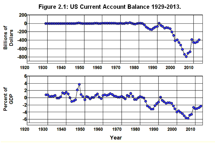
Source: Economic Report of the President, 2013 (B103PDF|XLS), Bureau of Economic Analysis (1.2.5).
The graphs in this figure clearly show the consequences of our international policies as we went from a relatively stable balance through 1980 to a $160 billion deficit in 1987 that amounted to 3.4% of GDP. This balance gradually adjusted through 1991 then fell precipitously to reach a record deficit of $804 billion in 2006, a deficit equal to 6.0% of GDP.
International exchange rates are supposed to adjust to eliminate this kind of imbalance, as they seemed to have in the 1980s, but, as was noted above, this will occur only if a country is not allowed to undervalue its currency in world markets over time. Figure 2.2 shows the Chinese yuan/dollar exchange rate from 1988 through the first quarter of 2014. Here is a classic example of how unregulated foreign exchange markets can fail to adjust as they are supposed to. Even though the trade deficit with China grew from $68.8 billion in 1999 to $372.7 billion through 2005, there was virtually no change in the yuan/dollar exchange rate in spite of this increase.
Source: Economic Report of the President: 2006 (B110PDF|XLS) OANDA .
It is worth emphasizing at this point that even though our trade deficit with China is three times that of our deficit with the rest of Asia, all of Europe, or with Latin America, the problem is not just with the yuan/dollar exchange rate. As should be clear from Figure 2.3, the entire structure of US exchange rates is overvalued today. The table in this figure shows the US balance of trade with its major trading partners and with the major trading areas of the world from 2001 through the third quarter of 2009. A clear indication of the degree to which the entire structure of US exchange rates is too high is given by the fact that the only entity in this table with which the United States has not had a consistent negative balance over this nine years is Singapore.
Source: Economic Report of the President, 2013 (B105PDF-XLS).
Undoubtedly, some of the deficits exhibited in this table can be explained by the growing need for U.S. dollars as international reserves held by foreign countries, but certainly not all. This situation is unsustainable, and the exchange markets will eventually adjust to correct this imbalance, but when this kind of imbalance is allowed to persist for any length of time, the eventual adjustment has the potential to precipitate a crisis that can lead to an economic disaster—a disaster that could have been avoided had this kind of imbalance not been allowed to occur in the first place. (Stiglitz Galbraith Reinhart Eichengreen Rodrik Bergsten)
Even more important is the fact that the persistence of this kind of imbalance has terribly destructive effects on our economy. The result of the unfair competition created by the overvalued US dollar has been the destruction of entire industries in the United States as much of the manufacturing sector of our economy has been outsourced to foreign lands. Particularly hard hit in this regard are the computer and consumer electronics industries. Equally disturbing is the fact that the technologies necessary to produce these goods have been shipped abroad as well. These technologies are essential to the increases in productivity necessary to improving our economic well being, but once the industries that embody these technologies are gone, they may be gone for a very long time. Even if the value of the dollar were to fall in the near future, it would take years to reconstitute many of these industries and to embed in the American economy the requisite capital and technologies needed to produce these goods. (Phillips Eichengreen Rodrik Palley)
The Overvalued Dollar and International Debt
The trade deficits cause by an overvalued dollar have another disturbing consequence. When we have a deficit in our balance of trade, the demand for dollars in the exchange markets to finance our exports is less than the supply of dollars made available in these markets through the purchase of our imports. This difference shows up as a deficit in our current account.[2.2] When such a deficit exists, foreigners end up accumulating more dollars than they need to purchase the amount of our exports they are willing to purchase at existing exchange rates.
At this point, foreigners have a choice: They can either refuse to accept more dollars at the existing exchange rates and, thereby, force our exchange rates down—thus, stimulating our exports and inhibiting our imports until a current account balance is obtained at a lower exchange rate—or they can use the excess dollars they are accumulating to purchase assets from Americans in the international capital markets. The assets purchased are essentially any asset an American is willing to sell for dollars but primarily consist of financial assets such as government and corporate securities.
The balance in the international capital market is referred to as our capital account balance, and this balance must, by definition, exactly offset our current account balance—that is, a deficit in our current account must, by definition, be offset by a surplus in our capital account that is exactly equal to the deficit in our current account. (Ott B103PDF-XLS)
When foreigners buy American assets in the international capital market, they are, in effect, investing in the United States. At the same time, to the extent these assets are government and corporate bonds, they are lending us money. To the extent these assets are not government and corporate bonds they must be corporate stocks, American businesses, real estate, or other nonfinancial assets in the United States. This means that the greater our current account deficit, the grater our capital account surplus must be, and, as a result, the current account deficits displayed in Figure 2.1 above indicate the rate at which we were driving ourselves into debt or selling our companies and other assets off to foreigners.
Figure 2.4 shows the Net International Investment Position of the United States from 1976 through 2013, both in terms of absolute dollars and as a percent of GDP, where Net International Investment is the difference between the value of the assets Americans own in foreign lands and the value of the assets foreigners own in the United States. It shows how the surpluses in our capital account that correspond to the deficits in our current account have accumulated. The extent to which this difference is made up of debt obligations—mostly corporate and government bonds—represents the net debt Americans owe to foreigners.
Source: Bureau of Economic Analysis ( 1.2.5). (1)
It is clear from this figure that there has been a fundamental change in our indebtedness to foreigners as a result of our free trade policies. Since 1976, our Net International Investment Position has gone from a positive $458 billion as measured in 2005 dollars (8.9% of our GDP) to a negative $2.3 trillion by 2010 (17.6% of our GDP). At the end of World War II the United States was the largest creditor nation in the world, but as a result of the over valuation of the dollar, this ended in 1985 when we became a net debtor to the rest of the world. As a result of our trade policies we have increased our net debt and sold off American assets to foreigners to the tune of some $2.7 trillion since 1984, and, in the process, we went from being the world's largest creditor nation to the world's largest debtor nation. (BEA XLS IMF)
Why Foreign Debt Matters
For a country to accumulate foreign debt as it runs a persistent trade deficit is not, in itself, a bad thing. The United States followed this course throughout the nineteenth century and into the twentieth, but throughout that period we used that debt to import capital goods and foreign technology. We invested in public education and other public infrastructure that led to tremendous increases in productivity in agriculture and manufacturing. We built national railroad and telegraph systems and created steel, oil, gas, electrical, automobile, and aviation industries. Our trade policies protected our manufacturing industries as our economy grew more rapidly than our foreign debt, and as Europe squandered its resources in senseless conflicts, by the end of World War I the United States had become a net creditor nation and the economic powerhouse of the world.
This is not the course we have followed over the past thirty years. We have exported rather than imported capital goods and technology, and, in return, we borrowed to import consumer goods. We invested less in our public education, transportation, and other public infrastructure systems than other countries have invested, rather than more. While we made huge advances in the electronics and computer industries over the last forty years, our trade policies are not protecting our manufacturing industries, and we have outsourced the manufacturing and technological components of these industries to foreign lands. As a result, our economy is not growing more rapidly than our foreign debt, and it is the United States that is squandering its resources in senseless conflicts.
This process of rising trade deficits can sustain itself only so long as foreigners are willing to lend us the dollars to finance these deficits. This situation is unsustainable, and when foreigners refuse to continue to do so—as eventually they must if our foreign debt continues to rise faster than our GDP—the existence of this debt makes us vulnerable to the same kinds of international financial crises faced by other countries that have found themselves in a similar situation. (Eichengreen Rodrik Galbraith Reinhart Philips Stiglitz Kindleberger Morris Klein)
The dramatic redistribution of income within our society, the breakdown of the fiduciary structure of our economic and political systems, the increasing prevalence and severity of speculative bubbles, and the dramatic deterioration of our net international investment position are all direct results of the economic policy changes that have led to the deregulation of our economic system over the past forty years.
All of these phenomena are interrelated, and they are also interrelated with two other phenomena we have experienced in the wake of these policy changes—namely, the dramatic increase in domestic debt and the rise in financial and economic instability.
Appendix on International Exchange
Exchange Rates and International Trade
The exchange rate between the American dollar and a foreign country's currency is nothing more than the price foreigners must pay in their currencies to purchase dollars. If the Chinese must pay 10 yuan to purchase one dollar of our currency, the YUAN/USD exchange rate will be 10y per dollar. Similarly, if the EURO/USD exchange rate is 0.75 euros per dollar that means that Europeans must pay 0.75e to purchase one dollar of our currency. In general, the higher our exchange rate the higher the price foreigners must pay in their currencies to purchase dollars; the lower our exchange rate the lower the price foreigners must pay in their currencies to purchase dollars.
This works in reverse, of course, when it comes to us buying foreign currencies. If the YUAN/USD exchange rate is 10y per dollar then we can purchase 10y for one dollar, which works out to a price of 10 cents per yuan. If the exchange rate is 5y per dollar we can only purchase 5y for one dollar, which works out to a price of 20 cents per yuan. In general, the higher the exchange rate the lower the price we must pay in our currency for a foreign currency; the lower the exchange rate the higher the price we must pay in our currency for a foreign currency.
Exchange rates are extremely important in determining the flow of international trade because if we wish to purchase goods from a foreign country we must pay for those goods in the currency of that country. Similarly, if foreigners wish to purchase goods from us they must pay us in dollars. As a result, the exchange rates between currencies determine the prices people must pay in their own currencies for the goods they import from other countries.
To see how this works, consider a bushel of wheat in China that costs 20y. If the YUAN/USD exchange rate is 10y per dollar, someone in the United States who wished to purchase a bushel of Chinese wheat has to come up with $2 to purchase the 20y necessary to pay the Chinese farmer in yuan. The dollar price of Chinese wheat in this situation will be $2/bushel. If, instead, the exchange rate is only 5y per dollar, the American purchaser has to come up with $4 to purchase the 20y needed to purchase this bushel of wheat. This means the dollar price of Chinese wheat will increase to $4/bushel even though the yuan price of wheat in China hasn't changed. In general, the higher our exchange rates the lower the prices in dollars we must pay for foreign goods; the lower our exchange rates the higher the prices in dollars we must pay for foreign goods.
Again, this works in reverse when it comes to the Chinese buying from us. If the price of a bushel of wheat in the United States is $3, and our exchange rate with China is 10y per dollar, someone in China who wishes to purchase a bushel of American wheat will have to come up with 30y to purchase the $3 needed to pay the American farmer in dollars, and the yuan price of American wheat will be 30y/bushel. But if our exchange rate falls to 5y per dollar the Chinese importer will have to come up with only 15y to purchase the $3 needed to purchase the American wheat, and the yuan price of American wheat will fall to 15y/bushel even though the dollar price of wheat in the United States hasn't changed. In general, the higher our exchange rates the higher the prices foreigners must pay in their currencies for our goods; the lower our exchange rates the lower the prices foreigners must pay in their currencies for our goods in their currencies.
The importance of exchange rates in determining the flow of imports and exports between countries should be clear from the above. If our exchange rate is 10y per dollar, it is not cost effective for the Chinese to purchase our $3/bushel wheat since the yuan price of American wheat is 30y/bushel and the yuan price of Chinese wheat is only 20y/bushel. But if the exchange rate is 5y per dollar, the yuan price of American wheat is only 15y/bushel, and the yuan price of Chinese wheat is still 20y/bushel. Thus, even though it is not cost effective for the Chinese to purchase American wheat if the exchange rate is 10y per dollar, it is cost effective for them to do so when the exchange rate is 5y per dollar, assuming, of course, that it costs less than 5y per bushel to transport wheat from the United States to China.
Similarly, if the exchange rate were 5y per dollar, it would not be cost effective for us to buy Chinese wheat since the dollar price of Chinese wheat would be $4/bushel, and it would only costs us $3/bushel to buy domestically produced wheat. But if the exchange rate were to increase to 10y per dollar, the dollar price of Chinese wheat would fall to $2/bushel, and we could save $1 per bushel by buying Chinese wheat instead of producing our own.
The point is that exchange rates play a crucial role in determining whether or not it is profitable for us to import goods from foreign countries or foreigners to purchase the goods we export: When our exchange rates go up, the dollar prices of goods produced in foreign countries go down, and it becomes more profitable for us to import foreign goods; when our exchange rates go down, the dollar prices of goods produce in foreign countries go up, and it becomes less profitable for us to import foreign goods. At the same time, when our exchange rates go up, the foreign currency prices of our goods in foreign countries go up, and it becomes less profitable for foreigners to purchase our exports; when our exchange rates go down, the foreign currency prices of our goods in foreign countries go down, and it becomes more profitable for foreigners to purchase our exports.
Exchange Rates, Wages, and International Trade
The wage rate is nothing more than the price of labor. As a result, the exchange rate determines the relative wages between countries in the same way it determines any other relative price between countries.
If the price of labor is 40y/hr in China and the exchange rate is 10y per dollar, it will cost us $4 to purchase the 40y that an hour of labor costs in China. This means that the dollar price of Chinese labor will be $4/hr. If the exchange rate is 5y per dollar, it will cost us $8 to purchase the 40y that an hour of labor costs in China, and the dollar price of Chinese labor will be $8/hr. Thus, an increase in the exchange rate will decrease the price of foreign labor in terms of dollars, just as it will decrease any other foreign price in terms of dollars, and a fall in the exchange rate will increase the price of foreign labor in terms of dollars, just as it will increase any other foreign price in terms of dollars.
This brings us to a very important point, namely, that just because the exchange rate is such that wages are lower in a given country (such as China) when measured in the same currency (either yuans or dollars) than they are in the United States, this does not mean that everything will be cheaper to produce in that country than in the United States. The reason is that the price of labor is only one of the factors that determine the cost of producing something. There are other costs as well, in particular, the costs of natural resources and of capital. In addition, the cost of labor does not depend solely by the price of labor. It also depends on the productivity of labor, that is, on the amount of output that can be produce per hour of labor employed.
The importance of this should become clear when we consider that, in spite of the fact wages are much lower in China than they are in the United States, we do not import wheat from China. The reason is that, in general, capital equipment is scarce and very expensive in China relative to labor, including the kinds of farm equipment we take for granted in the United States. The scarcity of capital equipment, in turn, means that much of the work that is done by capital equipment in the United States must be done by people in China to the effect that more labor is required to produce a given quantity of a good in China than is required to produce that same quantity of that good in the United States.
The fact that it takes more labor to produce a given quantity of wheat in China than it does in the United States means that the cost of labor in producing wheat is higher than the dollar price of labor indicates. In fact, when we combined the cost of labor in China with all of the other costs of producing wheat, including the cost of farm equipment, transportation, energy, taxes, etc. we find that, at the existing exchange rate, it actually costs more to produce a given quantity of wheat in China than it does in the United States. This is so even though the dollar price of Chinese labor is far below the dollar price of American labor. As a result, the price of Chinese wheat—which is determined by the total cost of producing wheat, not just the price of labor—when measured in dollars at the existing exchange rate, is higher than the dollar price of wheat in the United States, and we do not import wheat from China. Instead, China imports wheat from us.
It is the dollar prices of foreign produced goods relative to the dollar prices of domestically produced goods that determines which goods we import from foreign countries and which goods foreign countries import from us, not the dollar prices of labor. And the fact that these relative prices are determined by exchange rates means that in order to understand how imports and exports are determined, we must look at how exchange rates are determined between countries as well as how prices are determined within countries. (Smith)
The Foreign Exchange Market
Since a country must pay for the goods it imports in the currencies of the countries in which its imports are produced, a country’s imports must be financed in the foreign exchange market, that is, in the market in which the currencies of various countries are bought and sold. The most important source of demand in this market comes from foreigners who purchase a country's currency in order to obtain the exchange needed to purchase the country's exports. Similarly, the most important source of supply comes from a country's importers who sell the country's currency in order to obtain the foreign exchange needed to finance imports.
When the value of a country's imports is equal to the value of its exports it can obtain enough foreign exchange in the foreign exchange market to finance its imports from the sale of its exports. But if the value of its imports exceeds the value of its exports there will be a deficit in its balance of trade, and it will not be able to finance all of its imports in this way. This deficit must be financed, and one of the ways it can be financed is from income earned by individuals and institutions in the country on the investments they have made in foreign countries that are denominated in the foreign currencies.
When individuals or institutions in a country own earning assets that are denominated in foreign currencies, the earnings on those assets can only be spent in the domestic economy if they are converted into the domestic currency in the foreign exchange market. As they are converted, they contribute to the supply of foreign exchange available to that country. By the same token, when individuals or institutions in foreign countries own earning assets that are denominated in a country's domestic currency, the earnings on those assets can only be spent in the foreign countries if they are converted into foreign currencies in the foreign exchange market. As they are converted, they contribute to the country's demand for foreign exchange.
A similar situation exists when individuals or institutions simply transfer funds abroad. When an individual sends money to a family member abroad or a business transfers funds to a foreign subsidiary or a government provides aid to a foreign country in the form of cash it increases the demand for the foreign currency and the supply of the domestic currency in the foreign exchange market as those funds are converted into foreign currencies by their recipients. As a result, these kinds of international transfers of funds contribute to the supply and demand in the foreign exchange market in the same way international payments of income contribute to the supply and demand in this market.
A countries net exports—that is, difference between its exports and its imports—plus its net income (similarly defined) on foreign investments plus its net transfers of funds is referred to as the country's current account balance. The significance of this balance is that it defines the extent to which a country is able to pay for its current imports, current transfers of funds abroad, and current income earned by foreigners who hold earning assets denominated the country's currency out of the foreign exchange it receives from the sale of its current exports, receipt of current transfers of funds from foreigners, and its income received from holdings of earning assets denominated in foreign currencies.
The composition of the current account balance for the United Sates from 1929 through 2013 is shown in Figure 2.5. The extent to which our Current Account Balance has been dominated by our balance of trade (Net Exports) is clear in this figure. Only during the Marshall Plan following World War II have they differed significantly.
Source: Bureau of Economic Analysis (4.1)
When a country's current account is balanced all of its current international expenditures can be financed by its current international receipts of foreign exchange, where its current expenditures and receipts are those that are generated through the ordinary process of producing goods and earning income in the international economic system. When there is a deficit in a country's current account all of the country's current international expenditures cannot be financed through its current receipts, and when there is a surplus in a country's current account the country receives more than enough foreign exchange from its current receipts to finance its current international expenditures.
By definition, one country's current account deficit is some other country's current account surplus, and countries with deficits must must finance those deficits if their current account obligations are to be met. Since current account deficits cannot be financed through the ordinary process of producing goods, earning income, and international transfers, the only way they can be financed is through a transfer of assets from surplus countries' to deficit countries. These asset transfers are referred to as international capital flows, and they represent a willingness of foreigners in surplus countries to invest in deficit countries—either directly by purchasing real assets in the country or indirectly by purchasing the country's financial obligations, usually bonds or other forms of debt. Foreign investments of this sort can be used to finance a deficit in a country's current account because foreigners must pay for these investments in the deficit country's currency just as they must pay for the deficit country's exports in its currency.
As is explained in the text, a deficit in a country's balance of trade or in its current account is not, in itself, a bad thing, but there are two potential problems when it occurs. The first arises from the fact that while decisions regarding imports and exports tend to progress relatively slowly over time, the purchase and sale of financial assets in international markets can be executed almost instantly. This can lead to serious instability in the markets for foreign exchange as speculation and the concomitant speculative bubbles that culminate in financial panics and economic crises are accompanied by, and are often the result of, dramatic shifts in international capital flows.
The second potential problem that can arise when foreign investment is used to finance trade deficits has to do with the way in which these investments can be used to manipulate exchange rates. If a country with a trade surplus is willing to make foreign investments it can accumulate assets in deficit countries and, thereby, prevent its exchange rates from rising (deficit countries' exchange rates from falling). This makes it possible for the surplus country to keep the demand for its exports from falling in response to its surplus. The risk in doing this is that, because the assets being accumulated are denominated in foreign currencies, those who accumulate foreign assets in this way will take a capital loss on these assets in terms of their own currency if and when its exchange rates eventually rises (foreign rates fall) since these assets will then be worth less in terms of the domestic currency of the surplus country.
It is worth noting, however, that this potential for capital loss is not necessarily a deterrent to a country artificially suppressing its exchange rate in this way. To the extent the accumulated foreign assets can be transferred to the country's central bank or to its government, it is the central bank or government that will take the capital loss when exchange rates eventually adjust rather than those who earn their incomes in the exporting industries or otherwise benefit from the lower exchange rate. In addition, as is noted in Chapter 3, a trade surplus makes it possible for the distribution of income to be concentrated at the top of the income distribution in that when a country has a surplus in its balance of trade, full employment can be maintained with a higher concentration of income than in the absence of a trade surplus. It is also worth noting that, as is apparent from Figure 2.3, almost all countries have been willing to take this risk vis-à-vis the American dollar in recent years in order to build up their international reserves, stimulate their economies, or maintain the concentration of income within their societies.
Allowing countries to prevent their exchange rates from rising and, thereby, keeping our exchange rates from falling has led to our exchange rates being overvalued in the market for foreign exchange for most of the past thirty years as foreign countries have accumulated surpluses in their balance of trade while we have accumulated deficits in ours. As a result, foreign goods have been undervalued in our domestic markets for most of the past thirty years which has given importers an unfair, competitive advantage in these markets. This has placed a serious drag on the American economy and has had a particularly a devastating effect on our manufacturing industries. In addition, as we will see in Chapter 3, to the extent this drag has contributed to the need for a rising debt to maintain employment, it has also contributed to the instability of the American economy.
Endnote
[2.1] See the Appendix on International Exchange at the end of this chapter for a discussion of what it means for the dollar to be overvalued and for an explanation of international exchange rates, financial markets, and the relationship between international trade and capital flows.
[2.2] That is, to the extent this deficit is not offset by net foreign income/transfers. See Appendix: The Foreign Exchange Market at the end of this chapter.
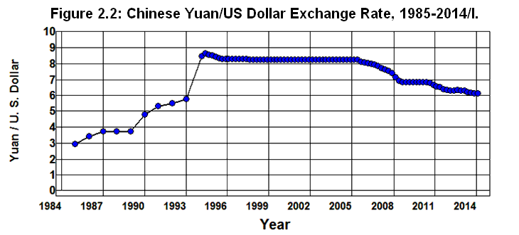
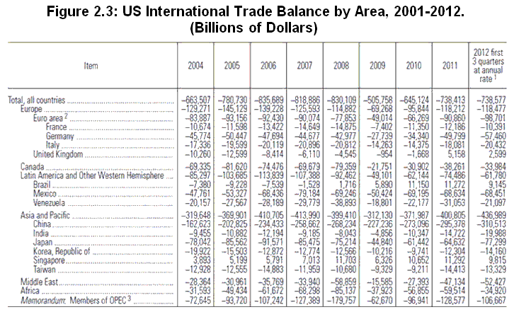
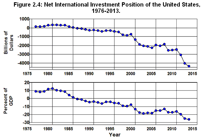
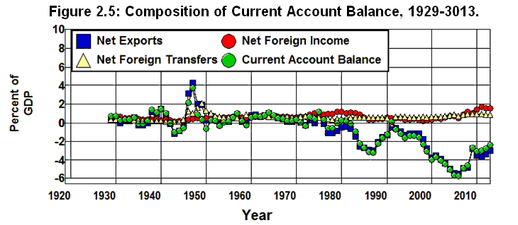
Chapter 3: Mass Production, Income, Exports, and Debt
George H. Blackford © 2009, last updated 5/16/2014
The history of economic development over the past four hundred years has been one of ever increasing output throughout the world as productivity increases in agriculture, textiles, steel, transportation, manufacturing, and, in today's world, automation, communication, and information technologies have been made possible through specialization, the division of labor, and the development of other mass-production technologies.
The concept of interchangeable parts along with technological advances in the machine-tool, steel, and transportation industries, combined with the use of assembly-line techniques and the development of electrical power and other utilities have led to a literal explosion in manufacturing since the beginning of the twentieth century. Automobiles, airplanes, farm and industrial equipment, construction materials, electronic equipment, home appliances, power tools, medical equipment and supplies, drugs, furniture, clothing, meat packing, fast foods, canned goods and other processed foods—virtually all of the goods the vast majority of the people spend the bulk of their incomes on today and many of the services, such as big-box retail, financial, and distribution services, as well—have proved to be amenable to the mass-production techniques that were developed or refined in the last century.
The process of technological advance and the development of mass-production techniques holds the potential for dramatic improvements in the economic wellbeing of the world’s population as ever greater quantities of goods can be produced with ever smaller amounts of human effort, but there is a catch: In order to be economically viable, mass production techniques require mass markets—that is, markets with large numbers of people who have purchasing power. Otherwise, the mass quantities of goods and services that can be produced via mass-production techniques cannot be sold. The existence of mass markets within a society, in turn, depends crucially of the distribution of income within that society: The less concentrated the distribution of income, the larger the domestic mass market will be; the more concentrated the distribution of income, the smaller the domestic mass market will be.
This brings us to the crux of the problem endemic in the changes in the distribution of income that have taken place during the past thirty years, namely, that the share of income that went to the top 1% of the income distribution in the 2000s was twice what it was in the 1960s and 1970s.
Doubling the income share of the top 1% from approximately 8% in 1980 to 18% in 2007 means the share of the bottom 99% went from 92% to 82%. As a result, the bottom 99% of the income distribution—99 out of 100 families—had, on average, 11% less purchasing power from income relative to the output produced in 2007 than the bottom 99% had relative to the output produced in 1980, and as we go down the income scale the reduction in purchasing power from income becomes more dramatic. The World Top Incomes Database shows that the fall in income for the bottom 90% of the income distribution from 1980 to 2007 was 20%. This means that in 2007 the bottom 90% of the population—9 out of 10 families—had, on average, 20% less purchasing power from income relative to the output produced in 2007 than the bottom 90% had in 1980 relative to the output produced in 1980.
Exports and Imports
In addition to the decrease in domestic purchasing power from income relative to the output produced experienced by the vast majority of the population since 1985, a substantial portion of the remaining purchasing power generated through the production of goods and services has been siphoned off by an increase in imports relative to exports.
As can be seen in Figure 3.1, until 1983 the United States Current Account Balance barely exceeded 1% of GDP other than in the aftermath of World War II. As a result, changes in imports and exports played a relatively minor role in the development of mass-production markets in the United States throughout most of the twentieth century. This changed after 1982 as our current account deficit (i.e., negative Current Account Balance) grew. While exports remained essentially unchanged from 1980 through 2007, going from 9.8% to 11.5% of GDP, imports increased from 10.3% to 16.4% of GDP. As a result, our Current Account Balance went from a 0.3% of GDP surplus to a 4.8% deficit.
Source: Bureau of Economic Analysis (4.1 1.1.5)
One would expect this kind of structural change, when combined with the increased concentration of income, to have a disruptive effect on employment and output as prices and profits fell in those areas that compete with imports and serve mass markets while prices and profits increased in those areas that serve the top 1% of the income distribution. But it would seem that the increase in income concentration and imports has had little effect on the viability of our domestic mass markets. There has, of course, been a rather devastating effect in the manufacturing sector of our economy as the decline in the rust-belt states can attest, but in spite of the losses in manufacturing and the three minor recessions we experienced from 1980 through 2006, unemployment and inflation trended downward over the period as employment and productivity rose. At the same time, mass market retailers such as Wall-Mart and Home Depot seem to have thrived.
The purchasing power necessary to maintain domestic output and employment in our mass-production society had to come from somewhere as the incomes of the vast majority of the population fell relative to the ability to produce and imports rose relative to exports from 1985 through 2006. Given the circumstances, the only place from which it could have come was through the transfer of purchasing power from those who had it and did not wish to purchase newly produced goods and services in the quantities needed to maintain our mass-production economy to the vast majority of the population that was losing purchasing power and was willing to purchase newly produced goods in the quantities needed to maintain our mass-production economy. This is especially so in view of the almost continuous increase in productivity that occurred since 1980.
100 Years of Income, Debt, and Economic Instability
The primary mechanism by which purchasing power is transferred from those who do not wish to spend to those who do wish to spend is through the creation of debt, that is, by those who have purchasing power and are unwilling to use it lending to those who are willing borrow in order to use it.[3.1] To the extent borrowed money is used to purchase newly produced goods and services that would otherwise not have been purchased, an increase in debt leads to an increase in the demand for goods and services. In so doing, increasing debt provides a mechanism by which it is possible to maintain mass markets and full employment as productivity increases, income becomes more concentrated, and imports increase relative to exports without the need for prices to adjust to redistribute income[3.2] or for exchange rates to adjust to reduce imports relative to exports.
The point is, given the state of mass production technology within our society, the domestic markets necessary to support full employment could not have been maintained without an increase in debt as the income transfer to the top 1% and 10% of the income distribution examined in Chapter 1 took place and, thus, diluted the purchasing power of the rest of the population relative to the output produced. This is especially so as the situation was made even worse as imports of mass produced goods increased relative to exports and productivity increased. Since employment, output, and productivity all increased during this period, it should not be surprising to find that debt increased dramatically as well.[3.3]
The dramatic changes that have occurred in the concentration of income and the growth in debt since 1913 are shown in Figure 3.2 which plots the income share received by the Top 1% of the income distribution through 2012 as well as Total Debt, Non-Federal Debt, and Federal Debt outstanding in the United States from 1916 through 2013. These changes have had profound effects on the development of mass markets and the utilization of mass-production technologies within the economic system throughout the twentieth century. They have also had profound effects on economic instability.
Source: The World Top Incomes Database, Federal Reserve (L1), Historical Statistics of the U.S.
(Cj870 Ca9-19), Bureau of Economic Analysis (1.1.5).[3.4]
Turn of the Century Through the Great Depression
The expansion of mass production undoubtedly received a huge boost from the increase in Exports and the expansion of Federal Debt that accompanied the 1914 outbreak of World War I That boost proved unsustainable, however, as the economy entered the 1920-1921 recession at war's end. This recession was followed by a speculative bubble in the real-estate market that was superseded by a speculative bubble in the stock market.
As can be seen in Figure 3.2, these two bubbles were accompanied by an increase in both debt and the concentration of income as Total Debt went from 156% of GDP in 1920 to 192% in 1928 and the income share received by the Top 1% went from 14.5% of total income (excluding capital gains) to 19.6% in those eight years.
The expansion of debt that offset the concentration of income in the 1920s not only allowed the markets for mass-produced goods to grow with the economy during that decade,[3.5] as we will see in Chapter 4, it also made these markets increasingly vulnerable to an economic downturn and, in the process, undermined the stability of the financial system. As a result, when the economic downturn began in the summer of 1929, and the stock market crashed in the fall of that year, the financial system began to founder. The absence of deposit insurance combined with an unwillingness (or inability) of the Federal Reserve to prop up the banking system led to a run on the system in the fall of 1930 that caused the financial system to implode. This worsened the economic downturn as the economy spiraled downward from 1929 through 1933. (Meltzer, Friedman and Schwartz, Fisher, Skidelsky Eichengreen Kindleberger)
The phenomenal fall in wages, prices, output, and income that resulted caused Total Debt as percent of GDP to increase from 184% of GDP in 1929 to 295% by 1933. As we will see in Chapter 15, this dramatic increase in the debt ratio was caused by the 45% decrease in GDP that occurred during this period, rather than by an increase in debt. Total debt actually fell by 12% from 1929 through 1933. In the meantime, over 10,000 banks failed along with 129,000 other businesses; the unemployment rate soared to 25% of the labor force, and 12 million people found themselves unemployed by the time the downward spiral of the economy came to an end in 1933.
This 283% debt ratio was, of course, unsustainable, and a massive deleveraging of the system took place as Total Debt as a percent of GDP fell from 295% in 1933 to 184% by 1940. As we shall see, again in Chapter 15, this deleveraging took place through the growth in GDP as unemployment fell and output and prices increased rather than through a fall in the debt itself which actually increased during this period.
Even though GDP managed to increase by 80% from 1933 through 1940, the actions of the federal government were too little and too late to maintain the mass markets necessary to keep output from falling dramatically through 1933 or to bring the system back to full employment before 1942. Federal Debt more than doubled, and even though the income share ae the Top 1% fell substantially from its 1928 high of 19.6%, it remained above 15% in all but one year during the 1930s. The rate of unemployment remained above 14% for the entire decade following 1930 and, as is shown in Figure 3.3, did not fall below 14% until 1941.
Source: Bureau of Labor Statistics (1), Economic Report of the President, 1960 (D17).
World War II and its Immediate Aftermath
The decade of the 1940s was dominated by World War II as the federal government took over the economy. Not a single automobile was produced in the United States from early in 1942 through 1945, and production of other consumer durable goods was suspended as well. Government mandated wage and price controls were instituted, and consumer goods were rationed as every effort was made to direct our economic resources into the production of war materials. The massive increases in government expenditures this entailed, combined with the extraordinary increase in the size of the military, brought the economy to near full employment in 1942 and to extraordinarily low levels of unemployment from 1943 through 1945. In addition, taxes were increased substantially as the top marginal tax rate was eventually set at 94%. (Kennedy)
In spite of the dramatic increase in Federal Debt during the war—from 44% of GDP in 1941 to 111% by 1945—Total Debt as a percent of GDP hardly increased as it went from 163% to 178%. This feat was accomplished through a massive deleveraging of the non-federal sector of the economy as wage and price controls and rationing combined with the tremendous increase in production, hence, income, made it possible for the ratio of Non-Federal Debt to GDP to fall from 120% of GDP in 1941 to just 67% by 1945. This fall in Non-Federal Debt set the stage for what was to follow.
The Prosperous Years: 1950 through 1973
The economy did not suffer the fate at the end of World War II it had suffered at the end of World War I. A massive demobilization took place as our factories retooled from the mass production of war materials to the mass production of civilian goods, and millions of service men and women were discharged from the military, but there was no major recession, and, as can be seen in Figure 3.3, unemployment remained below 6% for twelve years following World War II and below 7% until 1975.
The fact that Europe and Asia were devastated by the war aided the transition to a peacetime economy in that the need to rebuild the war-torn countries caused Exports (Figure 3.1) to remain high during the four years following the war. At the same time, government policies, such as the GI Bill, helped to ease the transition from military to civilian life for millions of veterans as they mustered out of the service.
Federal Debt decreased almost continuously relative to GDP following World War II, form a 1945 high of 111% of GDP to its post-war low of 23.1% of GDP in 1974—a fall of 88 percentage points. Total debt, on the other hand, increased gradually relative to GDP from 1951 through 1981, going from 129% of GDP to 165%. This increase of 36 percentage points in total debt took place in spite of a 44 percentage point decrease in Federal Debt over that 21 year period. The reason is that while Federal Debt relative to GDP was decreasing over this period, it was decreasing at half the rate at which Non-Federal debt was increasing. Non-Federal debt went from 67% of GDP in 1951 to 139% in 1981—a 72 percentage point increase that more than offset the 44 percentage point fall in Federal Debt.
While there was a relatively large increase in Non-Federal Debt through 1975, that debt was sustainable in that it was not backed by investments based on speculative bubbles or on consumers’ incomes created by speculative bubbles. It was backed by profitable investments both in the private and public sectors of the economy—investments in private capital and public infrastructure that increased productivity sufficiently to be self financing—and by consumers’ incomes that were derived from the employment created by those profitable investments.
Given the financial regulatory system put in place in the 1930s, the fall in income share of the Top 1% throughout the 1950s and 1960s (from 11.4% of total income in 1950 to 7.7% in 1973) made it possible for domestic mass markets to grow with the economy in such a way as to support the increases in mass production and productivity that took place during this period with relatively full employment and without an expansion of exports relative to imports. As a result, the domestic economy was able to grow and the vast majority of the population was able to prosper without creating the kinds of speculative bubbles that led to the economic catastrophe of the 1930s even though the expansion of domestic markets were aided by an expansion of debt.
The Great Inflation
The latter half of the 1960s through the first half of the 1980s—an era dubbed The Great Inflation by Allen Meltzer—presented a unique challenge to economic policy makers. From 1952 through 1965 the effective annual rate of inflation was 1.72%. From 1965 through 1984 it was 5.96%, and from 1975 through 1981 it was 7.66%. Efforts to end the inflation along with the 1973 Arab oil embargo and the concomitant quadrupling of the price of oil led to a number of shocks to the economic system. The turmoil of the times was reflected in a sharp fall in the growth of output in 1967, and a series of recessions that occurred in 1970, 1973-1975, 1980, and 1981.
The rise in interest rates combined with the 1980 and 1981 recessions that resulted from the efforts by the Federal Reserve to bring the inflation to an end left thrift institutions in desperate straits, but this did not pose a serious threat to the economic system itself. The existence of deposit insurance made it possible to avoid a run on these institutions and this allowed time to resolve the problem in an orderly way. The real threat to the system came from the changes in economic policies that took place in the 1980s in response to the problems caused by inflation and the energy crisis of the 1970s.
Reagan's Revolution
The results of the policy shift that took place in the 1980s are reflected in Figure 3.2 by the increase in Total Debt as a percent of GDP from 164% in 1981 to 231% by 1990 as the ratio of Federal Debt to GDP increased by 16 percentage points and that of Non-Federal Debt by 51 percentage points. The 67 percentage point increase in Total Debt that took place during the 1980s was six times the average for the previous three decades, and it not only fueled speculative bubbles in the commercial real-estate markets that brought on the savings and loan crisis in the 1980s, it also funded the hostile takeover/junk bond bubble that helped to create the current account deficits shown in Figure 3.1 that contributed to the decline of our manufacturing industries.
What is of particular interest here, however, is how the increase in debt made it possible for unemployment to trend downward over the decade in spite of the fact that imports rose and then fell relative to exports and the concentration of income that went to the Top 1% of the income distribution increased from 8.2% of total income in 1980 to 13.0% by 1990.
The Go-Go 1990s
The 1990s began with a minor recession as the unemployment rate reached 9.7% of the labor force in 1992, up from 5.3% in 1989. Income concentration was fairly stable from 1988 through the first half of the 1990s as the share of the Top 1% went from 13.2% in 1988 to 12.9% in 1994. Following 1994, however, there was a significant increase in concentration as the share that went to the Top 1% reached 16.5% by 2000. This was above where it had been in the early 1920s when the speculative bubbles began and above where it had been in all but two of the years our economy had stagnated through the 1930s when there were no speculative bubbles or wars to stimulate the economy.
There was some deleveraging that took place in the non-federal sector of the economy in the first two years of the 1990s, and then Non-Federal Debt continued upward at a steady pace until it began to increase more rapidly following 1997. In the meantime, Federal Debt peaked at 48.5% of GDP in 1993 and declined to 31.8% of GDP by 2001 as Total Debt went from 231% of GDP in 1990 to 265% by 2000.
At the same time, there was a dramatic increase in imports relative to exports as the deficit in our Current Account went from 1.3% to 4.0% of GDP. (Figure 3.1) In addition, productivity increased dramatically as the average increase in output per hour during the last half of the 1990s was almost twice that of the average increase for the previous ten years. All of these factors would have made it difficult, if not impossible, to maintain the domestic mass markets needed for full employment in the absence of the 33 percentage-point increase in Total Debt that took place during that period as unemployment fell from 7.5% of the labor force in 1992 to 4.0% in 2000.
It is also worth noting that, by all accounts, financial wealth more than tripled in the five years from 1995 through 2000. The NASDAQ Composite Index went from a low of 791 in 1995 to a high of 5048 in 2000 as the Standard & Poor's 500 Index went from 501 to 1527. In the process, this unprecedented—except for the 1920s—increase in the value of stocks decreased the cost of equity capital for corporations, and thereby lowered the cost of financing investment through equity relative to the cost of financing investment through debt. At the same time, the fact that realized capital gains steadily rose from 3.0% of total income in 1995 to 9.7% in 2000 made it possible for many to increase their consumption or investment expenditures without having to rely on debt. Both of these factors would tend to bolster domestic markets by offsetting the effects of increasing imports and income concentration.
In addition, unlike the situation in 1980s, as we will see below, there was, in fact, a significant increase in the average real income that went to the bottom 90% of the income distribution from 1993 through 2000 in spite of the increase in the concentration of income at the top that took place during that period. In any event, times seemed prosperous after 1995 until the stock market crashed in March of 2000, and the trillions of dollars of illusory paper wealth that had been created by the stock market bubble began to evaporate.
Even though tens, if not hundreds of billions of dollars had been wasted in the development of worthless dotcom companies such as Webvan.com, Pets.com, and Flooz.com, and billions more had been wasted in companies such as Enron, Global Crossing, and WorldCom there was not a collapse in the financial system when the Dotcom Bubble burst comparable to what had taken place following the Crash of 1929. What was different about the increase in paper wealth generated by the stock-market bubble in the latter half of the 1990s is that, unlike the 1920s, and in spite of the fact that Total Debt had increased substantially leading up to the crash, the Dotcom Bubble was not financed directly through an excessive buildup of debt collateralized by stocks.
The reason is that since the Securities Exchange Act of 1934, the Federal Reserve has had the power to set the margin requirement on loans collateralized by stocks, that is, has the power to set the minimum down payment a buyer must put up when borrowing money to buy stocks. The margin requirement was 50% during the 1990s which limited the amount of money speculators could borrow using stocks as collateral to 50% of the value of the stock. In the 1920s the margin was as low as 10% in the unregulated markets of the times which allowed speculators to borrow as much as 90% of the purchase price when purchasing stock. Even though the Federal Reserve refused to increase the margin requirement on stocks to keep the speculative bubble in the stock market from growing during the 1990s, the existence of a 50% margin requirement on loans collateralized by stocks minimized the damage caused by the Dotcom Bubble bursting.
As a result, few defaulted on their loans when this bubble burst, and there was not a wave of distress selling of assets which, as we will see in Chapter 4, had occurred following the Crash of 1929. While tens of millions of people were adversely affected as trillions of dollars of wealth disappeared into thin air, the financial system remained intact, and the economic system survived fairly well with a relatively minor economic downturn as unemployment increased from 4% of the labor force in 2000 to 6% by 2003. And since there were no insured deposits involved, there was no government bailout of depositors with taxpayers' money as there had been in the savings and loan debacle of the 1980s, though the federal Pension Benefit Guarantee Corporation insurance program did take a hit.
Then came the speculative bubble in the housing market brought on by the unregulated securitization of subprime mortgages. Unlike the stock-market bubble of the 1990s, the housing-market bubble of the 2000s was financed directly through an excessive buildup of debt collateralized by mortgages.
Unregulated Finance in the 2000s
Following passage of the Financial Services Modernization Act in 1999 and the Commodity Futures Modernization Act in 2000, the era of unregulated finance reached its pinnacle in the first half of the first decade of the twentieth-first century. It was an era of abiding faith in the ability of freewheeling capitalism to solve our economic problems by allowing unfettered markets to allocate resources in their most efficient manner. This freedom from regulation was supposed to bring economic prosperity to all. As it turned out, it didn’t. Instead, as is shown in Figure 3.1 and Figure 3.2, the cowboy finance that resulted led to dramatic increases in Imports, a further concentration of income, and a dramatic increase in debt.
The income share of the Top 1% fell from 16.5% in 2000 to 15.0% in 2002 as the fallout from the recession took its toll, and then, following the Bush tax cuts, increased to 18.3% of total income by 2007—just 1.3 percentage points below the peak it had reached in 1928. At the same time, imports increased relative to exports as the deficit in our Current Account went from 4.0% to 4.9% of GDP, and Total Debt increased continuously from 2000 through 2008—from 265% to 353% of GDP, an 88 percentage point increase in just seven years. At this point Total Debt as a percent of GDP was excessive even by the standard set in 1933 after GDP had fallen by 40% from its 1929 high.[3.6] By 2007 the GDP stood at $14.5 trillion and the Total debt at $51.1 trillion!
Why the System Collapsed
Servicing a debt of $51 trillion out of an income of $14 trillion places a huge burden on the system through the transfer of income from debtors to creditors. Even an average interest rate as low as 3% would require a transfer equal to 11% of GDP when total debt is as high as 370% of GDP. An average interest rate of 5% would require a transfer equal to 18% of GDP. In terms of real money, a 3% average rate of interest on the total debt of $54 trillion that existed in 2008 would have required that $1.6 trillion/year be transferred from debtors to creditors. A 5% average rate of interest would have required a $2.7 trillion transfer.
Figure 3.4 shows the interest rates paid on triple-A rated corporate bonds (Aaa Bonds), Municipal Bonds, conventional Mortgages, and Prime Rate loans from 1940 through 2012. The graphs in this figure indicate that interest rates in the early 2000s were comparable to those in the 1960s when Total Debt was less than 150% of GDP. It should be obvious that a return to the interest rates of the 1970s or 1990s with Total Debt equal to 353% of GDP, as it was in 2008, would present a daunting challenge.
Source: Economic Report of the President, 2013 (B73PDF|XLS)
Even more important is the fact that Non-Federal Debt had risen to 321% of GDP by 2008. Unlike the federal government which has the constitutional right to print money, those entities that make up the non-federal sector of the economy—whether they are individuals, businesses, financial institutions, or municipal governments—must service their debt out of income. When they cannot service their debt out of income they must refinance. Barring the ability to refinance, the only options to which they can turn is to the dreaded distress selling of assets or to default on their financial obligations—the kind of selling of assets and defaults that, as we shall see in Chapter 4 through Chapter 6, lead to financial crises.
Non-federal debt of this magnitude makes the economic system extremely fragile, and when much of that debt is the product of financing a speculative bubble and backed by assets and incomes generated by that bubble, the situation is even worse. It should be no surprise that in the face of the debt that existed in the mid 2000s, it was the upturn in interest rates in 2005 and 2006 caused by the Federal Reserve's attempt to moderate the housing boom that brought the housing bubble to an end in 2006 and sent shockwaves through the financial system in 2007.
It should also be no surprise that the bursting of the housing bubble in the United States reverberated throughout the rest of the world. The rise of the failed nineteenth-century ideology of Laissez-faire/free-market Capitalism that led to the deregulation of our financial system at home was not an exclusively American phenomenon. It had been promulgated all over the world by institutions such as the International Monetary Fund in the name of the now infamous Washington Consensus. (Klein) The result was not only financial deregulation and a housing bubble in the United States financed by expanding debt, but in many countries in Europe and elsewhere around the world. As a result, the crisis that was to explode in the American financial system in 2008 was destine to create a worldwide economic catastrophe.
100 Years of Income and Unemployment
It is, perhaps, worth emphasizing the obvious at this point, namely, that the degree of concentration at the top of the income distribution is related to the income at the bottom, and both are affected by economic policies.
Figure
3.5 plots the concentration of income of the Top 1% of the income distribution and the average real income (measured in 2012 prices) received by the Bottom 90% from 1913/17 through 2012. The way in which economic policies have affected these variables over the past one hundred years can best be understood by examining the historical context in which these variables have changed.
Source: The World Top Incomes Database.
Turn of the Century Through the Great Depression
T
he income share of the Top 1% (excluding capital gains) in this figure averaged 16.9% of total income from 1917 through 1933 with a low of 14.5% in 1920 and a high of 19.6% in 1928. The average real income of the Bottom 90% averaged $9,447 during this period and fell from a high of $11,291 in 1917 to a low of $6,676 in 1920 but had increased back to $10,536 by 1929. It then plummeted to $6,940 from 1929 through 1933.When we look at the historical context within which these changes took place we find that they began with World War I, followed by a rather steep recession in 1920 and 1921, a real-estate bubble from 1922 through 1926, a Stock-market bubble from 1926 through the fall of 1929, and three years of recession in which the rate of unemployment increased from 3.5% in 1929 to 24.9% in 1933.
We also find that, except during World War I, this was an era of less government, lower taxes, and virtually no regulation, and it ended in the depths of the Great Depression at the beginning of the New Deal—that is, at the beginning of an era of more government, higher taxes, and more regulation.
The average real income of the Bottom 90% began to increase after 1933 but was essentially the same in 1940 ($9,862) as it had been in 1920 ($9,676) and was still significantly below where it stood in 1917 ($11,291). At the same time, the concentration of income of the Top 1% averaged 15.9% from 1933 through 1940 and fell below 15% in only one year during that period. Unemployment remained above 14% throughout that period.
World War II and its Immediate Aftermath
Figure 1 and Figure 2 also shows the effects of World War II and its immediate aftermath as the government took over the economic system, instituted wage and price controls, rationed consumer goods, and increased personal and corporate tax rates dramatically. The result was a dramatic fall in unemployment, and the concentration of income of the Top 1% fell from 15.7% of total income in 1940 to 11.4% by 1950. At the same time there was a dramatic increase in the average real income of the Bottom 90% from $9,862 in 1940 to $18,797 in 1950.
The Prosperous Years: 1950 through 1973
Over the 23 years following 1950 we see another dramatic increase in the average real income of the Bottom 90% as it went from $18,797 in 1950 to $34,956 in 1973. At the same time, the concentration of total income at the top decreased fairly consistently throughout this period, falling from 11.4% of total income in 1950 to 7.7% in 1973.
Unlike the period leading up to 1933, this was decidedly an era of higher taxes, more government, and more regulation of the economy.
As can be seen in Figure 3.6, government made a relatively minor direct contribution to output in 1929, as reflected in the National Income and Product Accounts. The direct contribution of All Governments (federal, state, plus local) to GDP was less than 10% in 1929. It didn't exceed 15% until the beginning of the New Deal in 1933, and it remained at about that level through the remainder of the 1930s as the average real income of the Bottom 90% increased from $6,940 in 1933 to $9,862 in 1940.
Source: Bureau of Economic Analysis (1.1.5)
In addition, taxes were exceedingly low prior to the 1930s. The maximum marginal personal income tax rate was 7% before World War I, and even though it was raised to 77% during the war it had been cut back to 25% by 1925 where it remained until 1931. The maximum corporate tax rate was 2% prior to World War I and was raised to 12% during the war where it essentially remained until 1932.
This changed dramatically in the 40 year period following the New Deal during which taxes and the direct contribution of All Governments to GDP increased dramatically as the average real income of the Bottom 90% increased fourfold, from $6,940 in 1933 to $34,956 in 1973.
For the 23 year period from 1950 through 1973 the direct contribution of All Governments to GDP averaged 22.8% as the real income of the Bottom 90% increased from $18,797 to $34,956. At the same time, the tax structure put in place during World War II was, for the most part, left in place. The top marginal personal income tax rate was 91% and the corporate rate was 52% until the 1965, Kennedy-Johnson tax cuts reduced these rates to 70% and 48%.
The increase in the direct contribution of All Governments to GDP not only represented a direct increase in output during this period, it also led to a direct increase in employment as employment by governments (excluding the military) increased from 9.8% of the labor force in 1950 to 15.5% in 1973. (Figure 4) The great bulk of this increase took the form of an increase in teachers, police officers, firefighters, public health and safety inspectors, and regulatory personnel.
Bureau of Labor Statistics, (A-1 B-1)
The increase in the direct contribution of All Governments also led to substantial increases in productivity as a result of government investments in public education and scientific research, public transportation (city streets, county roads, state and interstate highways, bridges, ports, and subway, bus, and rapid transit systems), public health, water and waste treatment facilities, and other forms of public infrastructure. In addition, government investments in our regulatory systems not only led to significant improvements in public health and safety during this period, they also kept the financial system from blowing up the economy—there were no speculative bubbles from 1933 through 1973 of the kind that lead to financial and economic crises.
It is clear from Figure 3.3 and Figure 3.5 through Figure 3.7 that this era of higher taxes, more government, and more regulation from 1950 through 1973 led to low unemployment (averaging 4.8% for the entire period and exceeding 6% in only two years) and a dramatic increase the average real income of the Bottom 90% of the income distribution.
It is also clear, or at least it should be clear, that the increase in real income at the bottom was one of the most important factors that fueled the economy during this period. It was the increase in income at the bottom that caused the increase in output from 1950 through 1973, not the other way around. There is just no way all of the automobiles and refrigerators and washing machines and air conditioners and TVs and the countless other mass-produced goods and services that were produced during this period could have been sold if the income of the Bottom 90% had not increased in the way it did.
Who would have purchased all that mass-produced stuff if the concentration of income at the top and the average real income at the bottom had, instead, regressed back to their trends from 1917 through 1940 shown in Figure 3.5?
What would it have taken to maintain a fully employed economy if, following World War II, the concentration of income at the top and the average real income at the bottom had reverted back to their trends leading up to the war?
The answer to the later question can be found by looking back to the era that preceded World War II—the speculative bubbles of the 1920s and the secular stagnation of the 1930s—during which the concentration of income at the top remained high and the average real income at the bottom failed to rise. This was a period that ended in a decade in which the rate of unemployment never fell below 14% and in which the unemployment problem was not solved until the government took over the economy during World War II.
The answer to the latter question can also be found by looking forward to the era that followed 1973 when the average real income at the bottom again failed to rise and the concentration of income at the top began to regain the ground it had lost since 1928.
The Great Inflation
Therate of unemployment was 5.6% in 1973. From 1974 through 1980 it averaged 6.8%, and in 1980 the actual rate of unemployment stood at 7.1%. Undoubtedly, these dismal unemployment statistics were partly caused by the episodes of tighter monetary policy that resulted from the tremulous efforts of the Federal Reserve to fight the inflation that was raging at the time, and partly by the reduction in the direct contribution of All Governments to GDP from 24.2% in 1967 to 20.6% in 1980. It is also fairly safe to say that the relentless war waged against cost push inflation during this period played a major role in determining these statistics as the average real income of the Bottom 90% fell from $34,956 in 1973 to $32,413 by 1980.
Then came the
Reagan Revolution with its mantra of lower taxes, less government, and deregulation.Reagan's Revolution
While many government programs were cut during the Reagan years, as a result of the anti-Soviet defense buildup, the direct contribution of All Governments to GDP barely budged, going from 20.6% of GDP in 1980 to 20.5% in 1988. Reagan's successes in lowering taxes (cutting the top marginal personal income and corporate tax rates from 70% and 48% in 1980 to 28% and 34%, respectively, by 1988) and deregulating the economy, however, did help to lower the unemployment rate to 5.3% by the time he left office as the commercial real estate and junk bond bubbles that led to the Savings and Loan Crisis grew. But this triumph was short lived as these bubbles burst and unemployment rose to 7.5% in 1992 in the wake of the ensuing 1990 recession.
The net effect of this episode was to increase the concentration of income of the Top 1% from 8.2% in 1980 to 13.5% by 1992 as the average real income of the Bottom 90% fell from $32,413 to $31,174 during this period.
The Go-Go 1990s
Then came the 1990s in which we saw 1) a rather small increase in the top marginal personal and corporate tax rates from 28.0% and 34.0% to 39.6% and 35.0%, respectively, 2) a significant cut in the direct contribution of All Governments to GDP from 20.6% of GDP to 17.8%, 3) a dramatic increase in our current account deficit from 0.7% of GDP in 1992 to 4.0% by 2000, and 4) an almost total emasculation of the regulatory systems within the federal government.
Aided by the largest stock-market bubble since the 1920s, the unemployment rate fell from 7.5% of the labor force in 1992 to just 4.0% in 2000 as the average real income of the Bottom 90% increased from $31,174 to $35,799, surpassing, for the first time, the $34,956 level it had achieved in 1973. This feat was accomplished in spite of a significant increase in the concentration of income of the Top 1% from 13.5% to 16.5% of total income.
Unfortunately, when the dotcom and telecom bubbles burst and the dust had settled from the resulting
2001 recession, by 2003 the rate of unemployment had increased to 6.0% of the labor force, and the average real income of the Bottom 90% had fallen back to $33,368 and was, again, below the level it had achieved in 1973.Unregulated Finance in the 2000s
Finally, we have the aftermath of the financial deregulation of the late 1990s where the unemployment rate fell from to 6.0% in 2003 to 4.5% in 2007, and the average real income of the Bottom 90% increased somewhat during this period, from $33,368 to $34,816, slightly below the $34,956 level it had achieved in 1973.
Then, in the wake of the housing bubble bursting in 2007 and the financial and economic systems melting down in 2008 the unemployment rate spiked to 9.6% of the labor force in 2010 and was still at 7.4% in 2013, six years after the recession began and in spite of a 4.2% fall in the labor force participation rate during this period.
But the real story of this era is the increase the income share of the Top 1% from 15.2% of total income in 2003 to 18.3% in 2007, falling to 16.7% in 2009 in the wake of the Housing Bubble bursting and then rebounding to 19.3% of total income by 2012—just 0.3 percentage points below the high of 19.6% it had achieved in 1928—while the average real income of the Bottom 90% fell from $34,816 in 2007 to $30,439 in 2012, a level not seen since 1967!
Summary
Just as it is clear from our historical examination of Figure 3.1 that the end result of the era of higher taxes, more government, and more regulation was low unemployment and a dramatic increase the average real income of the Bottom 90% of the income distribution, it is just as clear from our historical examination of this figure that the end result of the two eras of lower taxes, less government, and deregulation that we have experienced during the past one hundred years was speculative bubbles, sporadic and rising unemployment, and falling average income for the Bottom 90% of the income distribution.
These same results are embodied in Figure 3.8 which plots the average real income of the Top 1%, Top 5-1%, Top 10-5%, and the Bottom 90% of the income distribution from 1917 through 2012 on the same graph.
Source: The World Top Incomes Database.
There's something wrong with this picture, and it is fairly easy to see exactly what's wrong with it. As John F. Kennedy pointed out, the rising tide that lifts all boats comes from a flood of rising income at the bottom of the income distribution not from spouting geysers at the top.
Conclusion
Today we are faced with the same kind of situation we faced in the 1930s: Given the state of mass-production technology, the distribution of income is incapable of providing the domestic mass markets—that is, markets with large numbers of people who have purchasing power—needed to achieve full employment in the absence of a speculative bubble. If we do not come to grips with this problem our domestic markets for mass-produced goods will continue to erode, and we will be plagued with boom and bust cycles of economic instability that eventually lead to economic stagnation as we run out of speculative bubbles to stimulate the economy. It will be impossible to maintain the standard of living of the vast majority of our population in this situation as our economic resources are transferred out of those industries that produce for domestic mass markets and into those industries that produce for the privileged few. (King)
Not only will it be impossible to maintain the standard of living of the vast majority of our population if the concentration of income is not reduced, those at the top will eventually find they are getting a larger piece of an ever decreasing pie. It is domestic mass markets that make mass production possible, and it is mass production—made possible by our domestic mass markets—that made the United States the economic powerhouse of the world. The erosion of our domestic mass markets erodes the very foundation on which our economic system rests, and to the extent this foundation is undermined, our ability to produce is undermined as well. (Ostry)
The only way a country can take advantage of mass-production technologies in the absence of an income distribution that provides domestic mass markets capable of purchasing the output it can produced without increasing debt relative to income is by producing for export and running a current account surplus. Unfortunately, continually running a current account surplus leads to increasing the debts of foreigners relative to their incomes.
Increasing domestic debt relative to domestic income, or the debts of foreigners relative to their incomes is not sustainable in the long run. The transfer burden from debtor to creditor must eventually overwhelm the system and lead to a financial crisis that will cause the system to collapse. It is no accident that the current economic crisis began, and, at least so far, has hit the hardest those countries that were running substantial current account deficits in the face of speculative bubbles in their domestic economies.
Appendix on Estimating Debt
The Historical Statistics of the U.S. (Cj870 Ca9-19 provides estimates of total debt from 1916 through 1976, and the Federal Reserve's Federal Reserve's Flow of Funds Accounts (L1) provide estimates of total debt from 1945 through 2013, but the two series are only roughly comparable. For the thirty-one years in which they overlap, the Federal Reserve's estimates as a percent of GDP are systematically below the Historical Statistic's estimates by an average of 12%. Both sets of data are plotted individually in Figure 3.9.
Source: Federal Reserve (L1), Historical Statistics of the U.S. (Cj870 Ca9-19),
Bureau of Economic Analysis (1.1.5).In constructing Figure 3.2, the Historical Statistics' estimates were used to estimate Total Debt from 1900 through 1945 and the Flow of Funds' estimates were used from 1945 through 2012. The estimates from both sources are plotted for the year 1945, hence, the two points in the Total Debt and Non-Federal Debt curves in Figure 3.2 where Non-Federal Debt is obtained by subtracting Federal Debt from Total Debt in this figure. There was no need to make an adjustment if the Federal Debt and GDP series used in constructing this figure as the differences in the estimates provided by the Historical Statistics of the U.S. (Ca9-19) and the Bureau of Economic Analysis (1.1.5) in the years they overlap are insignificant.
When comparisons are made in the text between 1945 and years prior to 1945 the Historical Statistics value for 1945 will be used, and the Flow of Funds value will be used for comparing 1945 with subsequent years.
Endnotes
[3.1] The idea that income must be redistributed to take advantage of an increase in productivity may seem to be unorthodox to some economists, but the need for redistribution is, in fact, implicit within the standard competitive model that lies at the core of neoclassical economics. The distribution of income is simply assumed to adjust automatically to accommodate increases in productivity in this model as the system is assumed to remain at full employment and long run economic profits are competed away. In the real world, of course, the economic system does not stay at full employment and economic profits do not necessarily get competed away. As a result, there is no reason to believe that a society that exists in the real world will be able to take full advantage of an increases in productivity irrespective of the distribution of income since the distribution of income does not necessarily adjust in the real world the way it is assumed to adjust in the competitive model.
It should, perhaps, also be noted that since this model is typically presented in terms of a system of equations derived from the optimizing behavior of a typical household and a typical firm, the distribution of income is not even considered in this model, except by way of the assumption that the amount of income the typical household receives is determined by the quantities of productive resources it owns and the prices these resources are able to command in the marketplace. As a result, the standard model gives only a partial explanation of the distribution of income.
Since income is determined by the ownership of productive resources in this model, it is implicitly assumed that the distribution of income is ultimately determined by the distribution of wealth among households. This means that to examine how the distribution of income affects the economic system we must go beyond the system of equations that are derived from the optimizing behavior of the typical household and firm and consider how the distribution of wealth can be expected to affect the preferences of the typical household and how these preferences can be expected to affect the typical firm.
If the typical household is to describe a society that has a high concentration of wealth and, hence, income, it is reasonable to assume that the preferences of the household that typifies that society will favor those kinds of outputs that serve the wealthy few rather than those that serve a mass market and that the typical firm will employ technologies that produce these kinds of outputs most efficiently. By the same token, if the household is to describe a society that has a low concentration of wealth/income it is reasonable to assume that the preferences of the typical household will favor those kinds of outputs that serve mass markets and the typical firm will employ technologies that produce these kind of outputs most efficiently. There is nothing in the standard model that is inconsistent with these assumptions.
[3.2] It is, perhaps, worth noting that a simple regression of the income share of the top 1% on the ratio of Total Debt to GDP explains 88% of the variation in this income share from 1970 through 2008:
SIMPLE REGRESSION
P99-100 = 0.1041TotalD%GDP - 11.15CNST
COEF. SD. ER. t(37) P-VALUE PT.R SQ.
Debt%GDP 0.1041 6.295E-3 16.54 1.118E-18 0.8809
CNST -11.15 1.406 -7.93 1.696E-9 0.6296
R SQ. = 0.8809, ADJ.R SQ. = 0.8776, D.W. = 0.4462
SD.ER.EST. = 1.266, F(1/37) = 273.5 (P-VALUE = 1.118E-18)
If we add exports, imports, productivity, prices, and unemployment to the mix, the explanatory power of the regression reaches 97% with all of the coefficients significant at the 5% level and a Durbin-Watson statistic in the upper half of the indeterminate range:
MULTIPLE REGRESSION
P99-100 = 0.02401Debt%GDP + 0.4219Exports%GDP - 0.3851Imports%GDP + 0.07293Productivity + 0.03409CPI - 0.5343UnemployRate + 0.8225CNST
COEF. SD. ER. t(32) P-VALUE PT.R SQ.
Debt%GDP 0.02401 0.01055 2.275 2.975E-2 0.1392
Exports%GDP 0.4219 0.1336 3.159 3.446E-3 0.2377
Imports%GDP -0.3851 0.1535 -2.509 1.737E-2 0.1644
Productivity 0.07293 0.03353 2.175 3.712E-2 0.1288
CPI 0.03409 0.009314 3.66 9.004E-4 0.2951
UnemployRate -0.5343 0.08673 -6.161 6.824E-7 0.5426
CNST 0.8225 2.196 0.3745 7.105E-1 4.363E-3
R SQ. = 0.9746, ADJ.R SQ. = 0.9698, D.W. = 1.414SD.ER.EST. = 0.6282, F(6/32) = 204.7 (P-VALUE = 4.354E-24)
Source: Piketty and Saez(XLS), ERP, 2011(B1PDF|XLS B42PDF|XLS B49PDF|XLS B60PDF|XLS B69PDF|XLS B72PDF|XLS B104PDF|XLS), HSUS(Cj870-889). See footnote 3.3.
[3.3] The role of borrowing in this situation is explained quit succinctly by Cynamon and Fazzari:
The willingness and ability of the bottom 95% to borrow excessively that kept their demand growing robustly despite their stagnant income growth and sowed the seeds of the Great Recession. Without this borrowing, demand from the bottom 95% cannot come close to attaining the level necessary to reach full employment. Demand from the top 5% has continued to follow the pre-recession trend, but this is not enough. The problem is not so much that output produced by the rising productivity of the middle class is distributed to the upper class, who do not spend it. Rather, the problem is that absent either wage and salary growth or excessive borrowing by the middle class, the spending of the bottom 95% is inadequate to generate the demand growth necessary to push the economy toward full employment at an acceptable pace. A large share of the aggregate income that we could enjoy if our resources were fully utilized is never created at all due to inadequate demand.
It is worth noting, however, that the government's increase in borrowing leading up to the Great Recession had the same effect in increasing demand as borrowing by the bottom 95%.
[3.4] See the Appendix on Measuring Debt at the end of this chapter for an explanation of the way in which the data from the Historical Statistics of the U.S., Federal Reserve Flow of Funds Accounts, and Bureau of Economic Analysis are used in this figure.
[3.5] Robert Reich in his Aftershock: The Next Economy and America's Future provides the following quote form Marriner Eccles's Beckoning Frontiers, published in 1950, in which Eccles describes the forces that led to the Great Depression:
As mass production has to be accompanied by mass consumption, mass consumption, in turn, implies a distribution of wealth—not of existing wealth, but of wealth as it is currently produced—to provide men with buying power equal to the amount of goods and services offered by the nation's economic machinery. Instead of achieving that kind of distribution, a giant suction pump had by 1929-30 drawn into a few hands an increasing portion of currently produced wealth. This served them as capital accumulations. But by taking purchasing power out of the hands of mass consumers, the savers denied to themselves the kind of effective demand for their products that would justify a reinvestment of their capital accumulations in new plants. In consequence, as in a poker game where the chips were concentrated in fewer and fewer hands, the other fellows could stay in the game only by borrowing. When their credit ran out, the game stopped.
Robert Reich and Marriner Eccles are the only two individuals I have run across so far that seem to understand problem of a concentration of the distribution of income in a mass-production economy.
[3.6] It should be noted that these are only rough comparisons due to the differences in the way current and historical total debt is estimated. See the Appendix on Measuring Debt at the end of this chapter.
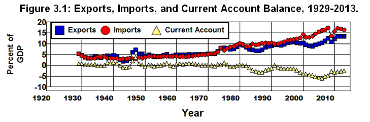
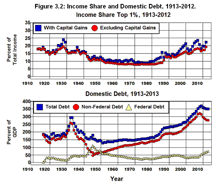
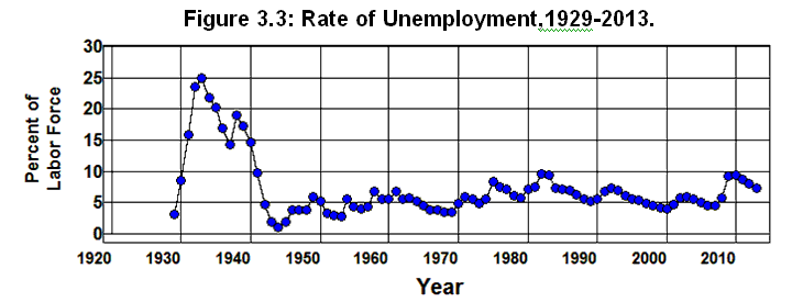
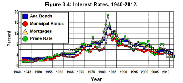
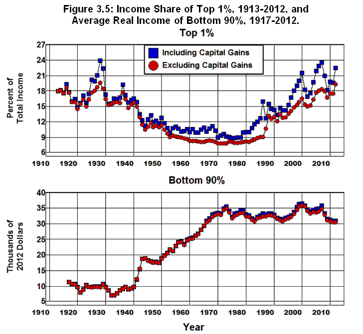
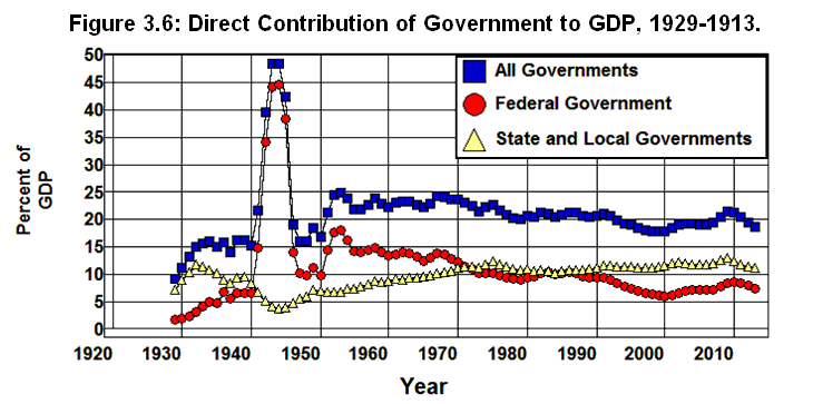
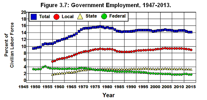
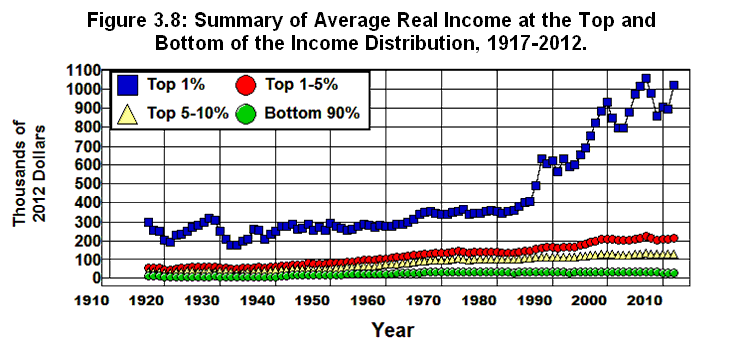
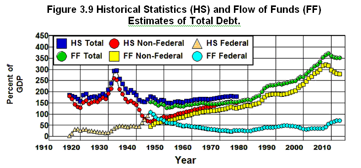
![]()
Chapter 4: Going Into Debt
George H. Blackford © 2009, last updated 5/1/2014
![]()
Figure 4.1 shows a breakdown of the public and private domestic debt in the United States from 1945 through 2013 in both absolute dollars and as a percent of GDP. As is shown in this figure, Total debt increased from less than $500 billion in 1950 to over $59 trillion by 2013 and, in the process, increased from 155% to 363% of GDP. It can also be seen that Federal Debt decreased rather consistently through the mid 1970s, and even though Federal Debt increased considerably after 1980 through (from $735 billion and 26% of GDP to $12.3 trillion and 74% of GDP by 2013), Federal Debt played a relatively minor role in the increase in the total. The major source of the increase in total debt following 1981 was in the non-federal sector of the economy.
Source: Federal Reserve (L1), Bureau of Economic Analysis (1.1.5).
The pattern of Non-Federal Debt increases displayed in Figure 4.1 is particularly telling. This debt increased from $1.3 trillion in 1970 to $46.6 trillion in 2008 and, in the process, increased from 121% of GDP to 321%. The increase was gradual until 1981 and then went from $4.4 trillion and 138% of GDP to $11.3 trillion and 189% in just 9 years. It dipped slightly relative to GDP in 1992 then increase dramatically over the next 14 years.
It is no accident that the dramatic jump in Non-Federal Debt from 1983 through 1990 followed on the heels of the Depository Institutions Deregulation and Monetary Control and Garn–St. Germain Depository Institutions acts being passed in 1980 and 1982. As was noted in Chapter 1, it was the deregulatory provisions in these acts that led to the first major financial crisis in the United States since the Crash of 1929. It is also no accident that the explosion of debt came to an end in 1990 on the heels of the savings and loan crisis or that Non-Federal Debt began to rise again in the mid 1990s.
Debt and Deregulation
The savings and loan crisis marked a minor setback in the movement to deregulate the financial sector. Congress to passed seven major pieces of legislation to reregulate the financial sector in response to this crisis .
The first was the Competitive Equality Banking Act in 1987 to recapitalize the Federal Savings and Loan Insurance Corporation (FSLIC), which was bankrupted by the crisis, and to strengthen the supervision in the savings and loan industry. Two years later Congress passed the Financial Institutions Reform, Recovery and Enforcement Act which transferred savings and loan deposit insurance from the failed FSLIC to the FDIC, reorganized and further strengthened the supervisory structure of the savings and loan industry, and created and funded the Resolution Trust Corporation to deal with the savings and loan institutions that had failed. (FDIC)
Next came the Comprehensive Thrift and Bank Fraud Prosecution and Taxpayer Recovery Act of 1990 to deal with the abusive practices of the new breed of savings and loan owners/managers, and in 1991 the Federal Deposit Insurance Corporation Improvement Act was passed. This act greatly increased the powers of the FDIC, put forth new capital requirements for banks, created new regulatory and supervisory examination standards, and established prompt corrective action standards that ostensibly took away some of the discretion of regulators when it came to dealing with insolvent institutions.
Finally, Congress passed the Home Ownership and Equity Protection Act of 1994 which dealt with abuses in the home mortgage market and gave the Federal Reserve the power to regulate this market.
These acts, combined with the enhanced vigilance on the part of regulators brought on by the savings and loan crisis, put an end to the explosion of domestic debt that accompanied the financial deregulation of the early 1980s. Unfortunately, this setback to the deregulatory movement was only temporary.
As the crisis wore on the general public failed to appreciate the seriousness of the situation. The reason is, the consequences of the crisis seemed to be relatively minor. There was a minor recession in 1990 that lasted into 1991, and the crisis cost the taxpayers some $130 billion, but there was no sense of panic at the near meltdown of the financial system. Deposit insurance prevented a run on the system, and the lives of relatively few people were seriously disrupted. At the same time, as was noted in Chapter 1, a relatively large number of people made personal fortunes out of this crisis. Since there was very little public outcry, very few lessons were learned, and there were virtually no political consequences for those who brought this crisis about.
The mantra of lower taxes, less government, and deregulation carried the Republican Party to victory in the 1988 presidential election in spite of the savings and loan debacle. What's more, the successes of the Republican Party throughout the 1980s had a profound effect on the leadership of the Democratic Party. A significant number of Democrats who opposed the free-market economic policies advocated by the Republicans either retired or were defeated at the polls. As a result, many Democrats began to embrace these policies—either out of conviction or to enhance their political survival. As the electorate shifted to the right on economic issues, the Democratic Party shifted to the right on these issues as well, and by the time of the 1992 election, opposition to financial deregulation was muted.
Bill Clinton held himself out as a "New Democrat" who embraced "values that were both liberal and conservative." He promised to reinvent "government, away from the top-down bureaucracy of the industrial era, to a leaner, more flexible, more innovative model appropriate for the modern global economy." When he became president he invited a number of ideologically minded economists to join his administration, three of which came to the fore: Alan Greenspan, Robert Rubin, and Lawrence Summers. (Turgeon)
Alan Greenspan was appointed by Ronald Reagan to chair the Board of Governors of the Federal Reserve and was reappointed to this position twice by Clinton. Robert Rubin was co-chairman of Goldman Sachs before Clinton selected him to chair the National Economic Council and then appointed him to replace Lloyd Benson as Secretary of Treasury. Lawrence Summers worked as an economist in the Reagan White House before he joined the Clinton Administration, first as Treasury Undersecretary for International Affairs and then as a replacement for Rubin as Secretary of Treasury. This is the triumvirate that dominated economic policy deliberations in the Clinton Administration—the group Time Magazine dubbed “The Committee to Save the World.” (Ramo Frontline)
There was little hope for financial regulation from this group. While the Home Ownership and Equity Protection Act was passed in 1994, its provisions giving the Federal Reserve responsibility for regulating the mortgage market were dutifully ignored by Greenspan, and the Riegle-Neal Interstate Banking and Branching Efficiency Act was passed that same year allowing interstate banking throughout the United States. Passage of this bill was particularly ominous in light of the fact that the Sherman Antitrust Act of 1890 and Clayton Antitrust Act of 1914—enacted to protect the public from anticompetitive practices on the part of businesses—had been virtually ignored since the Reagan Revolution began in 1980.
The spirit of deregulation got a further boost from the 1994 election. When the dust settled from that election Republicans had control of both the House and the Senate for the first time since 1954, and it was clear that the movement to reregulate the financial system was dead. A seemingly blind faith in free-market capitalism and deregulation became the tenor of the times. The extent to which this was so was made clear by Clinton in his 1996 State of the Union Address when he announced to the world that "the era of big government is over" and took pride in the fact that his administration had eliminated "16,000 pages of unnecessary rules and regulations."
On November 4, 1999, Congress passed the Financial Services Modernization Act (FSMA) which was signed into law by President Clinton on November 12. This act repealed those portions of the Glass-Steagall Act of 1933 that prevented commercial bank holding companies from becoming conglomerates that are able to provide both commercial and investment banking services as well as insurance and brokerage services. Congress then passed the Commodity Futures Modernization Act (CFMA) on December 14, 2000 which Clinton signed into law on December 21. This act explicitly prevented both the Commodity Futures Trading Commission and state gambling regulators from regulating the derivatives markets.
While the laws passed in the late 1980s and early 1990s led to stronger regulation of depository institutions, such as commercial and savings banks and savings and loans, by the mid 1990s the antiregulatory atmosphere in Washington made the enforcement of the new laws problematic, and, as we will see, passage of the FSMA and CFMA in 1999 and 2000 gave a free hand to investment banks, bank holding companies, hedge funds, and special purpose vehicles in the markets for repurchase agreements and financial derivatives. (See Chapter 8.)
The story of this era is reflected in Figure 4.1 which shows 1) the dramatic increase in Non-Federal debt as a percent of GDP following the deregulation of depository institutions and lax supervision on the part of regulators in the early 1980s, 2) the leveling off and slight fall in this debt as a percent of GDP in response to the reregulation of depository institutions and greater vigilance on the part of regulators in the late 1980s and early1990s, 3) the beginning of the increase in this debt in the mid 1990s as the regulatory attitude in Washington changed, and 4) the continuing increase in this debt ration from 2000 through 2008 following the passage of FSMA and CFMA. This same story is told in Figure 4.2 which shows the expansion of debt on the part of financial institutions over this same period.
Source: Federal Reserve (L1), Bureau of Economic Analysis (1.1.5).
Figure 4.3 shows what happened in the mortgage markets following the deregulation of the financial system in the 1980s. The increase in commercial mortgages as a percent of GDP that fueled the speculative bubble in the commercial real estate markets of the early 1980s is clearly visible in this figure, as is the collapse in this market following the bursting of this bubble. The increase in commercial mortgages that fueled the speculative bubble in the commercial real estate markets that accompanied the speculative bubble in the housing market during the early 2000s is also clearly visible in this figure, as is the collapse of this market following the crash of 2008.
Source: Federal Reserve (L2), Bureau of Economic Analysis (1.1.5).
Figure 4.3 also shows the dramatic increase in residential mortgages as a percent of GDP that took place during the commercial real-estate bubble in the 1980s and the huge increase that fueled the housing bubble in the 2000s along with the collapse of this market following 2007.
What Financial Institutions Do
It should not be surprising that the behavior of nonfinancial debt is related to the degree of regulation in the financial system. Creating debt is what financial institutions do.
Financial institutions provide the mechanisms by which borrowing and lending take place within society. In the process they provide other services such as insurance, a safe and convenient place to keep money, pension plans, and brokerage and underwriting services. They also deal in equities, that is, stocks as opposed to loans, bonds, mortgages, and other types of debt instruments. They underwrite the sale of newly issued equities and broker the purchase and sale of previously issued equities. They may also invest in equities, but the main business of finance is debt, not equities. Debt is where the money is. Without debt, there would be no financial system as we know it.
The primary mechanism by which financial institutions create debt is through the process of intermediation which means they intermediate between the ultimate borrowers and lenders in society. They take in money from the individuals and businesses that are the ultimate lenders and relend the money to individuals and businesses that are the ultimate borrowers. Banks take in money from their depositors who are the ultimate lenders and relend the money in the markets for consumer and business loans. Insurance companies take in money from their policy holders who are the ultimate lenders and relend the money in the mortgage and bond markets. Pension funds take in money from employees who are the ultimate lenders and relend the money in the mortgage and bond markets as well.
In addition, certain financial institutions, historically banks but, as we will see in Chapter 7, in today's world shadow banks as well, have the power to create debt out of thin air as a major portion of the money they lend is lent back to them to be relent again.
This process of intermediation is an essential part of the economic system, and without it the system cannot function. The problem is that while the ability for the economic system to function depends crucially on this process, in the absence of strict government regulation and supervision, this process is highly unstable. The reason this is so, and why these institutions must be regulated and supervised is obvious—financial institutions lend other peoples’ money. They take money from one group of people and lend it to another group of people as they take a cut in the process.
Not only does this process provide innumerable opportunities for fraud to flourish on a grand scale, there are powerful forces within society that drive the system of financial intermediation to fund speculative bubbles that increase debt beyond any possibility of repayment. The reason for this is also obvious—the more financial institutions are able to lend, the greater their cut, and the more money they are able to make. In addition, those in the financial system who handle other peoples’ investments have access to information that provides opportunities to profit from speculative bubbles in ways that are not available to those outside the system. (Stewart WSFC)
The simple fact is this: huge fortunes can be made by those who are able to take advantage of speculative bubbles. As was pointed out in Chapter 1, and worth repeating here, the extent to which the top 1% of the income distribution benefited from these bubbles is clearly shown in Figure 1.9 by the
53% increase in income share this group received during the 1921-1926 real estate bubble and the 1926-1929 stock market bubble that led up to the Great Crash of 1929 and the Great Depression of the 1930s.
55% increase in income share this group received during the 1981-1988 junk bond, and commercial real estate bubbles of the 1980s that led up to savings and loan crisis and the 1990-1991 recession.
51% increase in income share this group received during the 1994-2000 dotcom and telecom bubbles that led up to the stock market crash of 2000 and the 2001 recession.
39% increase in income share this group received during the 2002-2007 housing bubble that led up to the Great Crash of 2008 and the worldwide economic crisis we are in the midst of today.
Similarly, Figure 1.10 shows the amount of income received in the form of capital gains as a percent of total income from 1916 through 2010. The increase in capital gains by fully 6% of total income in the 1920s, 1990s, and 2000s depicted in this figure clearly shows the effects of speculation on income during these eras that led to economic catastrophes as those who profited from these bubbles realized huge capital gains. And again, Figure 1.11 shows the trillion dollars plus in additional profits reflected in the spike from 2001 through 2007 that financial institutions would not have made if there had been no housing bubble and their profits had stayed at their 2000 level.
It is no mystery why speculative bubbles persist in the face of such massive gains by those who are able to take advantage of these bubbles. The problem is, of course, that when those in charge of our financial institutions are allowed to finance speculative bubbles and increase debt beyond any possibility of repayment, they do not place only their own money and economic wellbeing at risk. They place other peoples' money and economic wellbeing at risk, and they threaten to bring down the entire economic system.
There are a host of powerful arguments, based on seemingly sound economic theory and irrefutable logic, put forth by those who favor deregulating markets to explain why unregulated financial markets lead to economic efficiency, growth, and prosperity, and why government regulation is the source of all problems, (Fox Taleb Dowd) but we are not talking about theory or logic here. We are talking about cold hard historical fact that goes far beyond what happened in the savings and loan crisis of the 1980s, the dotcom and telecom bubbles of the 1990s, and the housing bubble and sub-prime mortgage fraud of the early 2000s. We are talking about the economic catastrophes brought on by the financial crises in 1819, 1837, 1857, 1873, 1893, and 1907, and we are talking about the last time this happened in the United States—1929. (Fisher Keynes Polanyi Kindleberger Minsky Phillips Morris Dowd Reinhart Johnson Skidelsky Kindleberger Kennedy)
The Crash of 1929 brought an end to the Roaring Twenties with a vengeance, and the experience of the Great Depression that followed had a profound effect on the American psyche for the next fifty years. The story of the 2000s is very much the story of the 1920s—namely, extreme excess on the part of an unregulated financial system—and it is worth reexamining that story within the context of what we have experienced over the past forty years.
Those Who Cannot Remember the Past
The 1920s began with a rather steep recession in 1920-1921 followed by a speculative bubble in the real estate market. The real estate bubble burst in 1926 and was superseded by a speculative bubble in the stock market. There was a mild economic downturn in 1927, a brief recovery that same year, and another mild downturn in the summer of 1929. Then the stock market bubble came to a dramatic climax in the fall of 1929. (Galbraith Friedman Meltzer Kindleberger Eichengreen Kennedy)
The Crash of 1929 began on October 24—a day that became known as Black Thursday—when the stock market dropped dramatically in the morning and recovered somewhat in the afternoon. While prices rallied on Friday, there were two more black days to come. When trading resumed after the weekend, the Dow fell by 13% on Black Monday and it fell an additional 12% on Black Tuesday. There were rallies that followed, but, overall, the stock market lost 80% of its value from its high in 1929 to its low in 1932 and the Dow fell by almost 90%.
The Great Depression of the 1930s
As stock prices fell in the fall of 1929, the mild recession that had begun in the summer became severe, and a banking crisis began in the fall of 1930 that reached its climax in 1933 when some 4,000 banks and 1,700 savings and loans went under in that year alone. By the time the crisis came to an end some 10,000 banks had gone out of business along with 129,000 other businesses, and we were in the depths of the Great Depression.
From 1929 through 1933, unemployment went from 1.6 million to 12.8 million as the unemployment rate jumped from 3.2% of the labor force to 24.9%. The economy experienced a major deflation as consumer prices fell by 25% and wholesale prices by 30%. The total value of goods and services produced in the United States fell by 46%, the level of production fell by over 30%. Just as happened in 2008, the financial crisis in the United States spread throughout the rest of the world, and the entire world faced an economic catastrophe of epic proportions. (Kindleberger)
The depression lasted more than ten years. There were still 8.1 million people unemployed in 1940, and the unemployment rate did not fall below 14% until 1941. It wasn't until 1943—when the economy was fully mobilized for World War II—that the unemployment rate finally fell below its 1929 level, and by then the United States had increased the size of its military by over 8.5 million soldiers. In other words, we did not solve the unemployment problem created by the Great Depression until we were fully mobilized for World War II and had drafted a number of people into the military comparable to the number who were unemployed in 1940, though, obviously, there was a bit of overkill here when it came to solving the unemployment problem. (Figure 4.4)
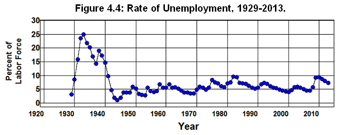
Source: Bureau of Labor Statistics (1), Economic Report of the President, 1960 (D17).
What Went Wrong
It was clear to most people at the time that the cause of the problem was rampant speculation in the stock market financed by expanding debt. In fact, the debt created by the financial system during the 1920s had grown to unreasonable levels in all areas, not just in the stock market. This debt was unsustainable, and the stock market crash was just the trigger that set in motion a set of forces that, in the face of this debt, brought down the entire economic system. (Fisher)
When the stock market crashed, the value of stocks that provided the collateral for speculative loans fell. This led to a panic in the financial sector as financial institutions tried to cut their losses by recalling existing loans and refusing to make new loans, not just loans collateralized by stocks but all loans. The financial system simply froze, and credit became unavailable. This forced debtors whose loans were called or who could not refinance their loans when they came due to sell the collateral underlying their debts as well as other assets in order to meet their obligations. These forced sales of collateral and other assets, in turn, caused asset prices to fall throughout the financial system, and debtors began to default as the value of their assets fell below the value of the loans they had to repay. (Fisher)
As the panic grew, businesses that were unable to finance their inventories and payrolls for lack of credit were forced to cut back their operations and layoffs began. At the same time, households that were unable to finance the purchase of such things as new homes, automobiles, and other durable goods for lack of credit were forced to cut back their expenditures. As output, employment, and business and household expenditures fell, income fell as well. The rise in uncertainty and the heightened sense of fear and pessimism toward the future exacerbated the situation. The result was a vicious spiral downward as falling output and employment led to falling income and expenditures which, in turn, led to falling output and employment. (Keynes)
All of this should sound familiar, given our experience during the current crisis, since this is exactly what happened in the mortgage market following the bursting of the housing bubble in 2007 and the financial system grinding to a halt in September of 2008.
Debt in the American economy had grown to unsustainable levels by 2007, and when the housing market crashed, the value of the real estate that provided the collateral for real estate loans began to fall. This led to a panic in the financial sector as financial institutions tried to cut their losses by recalling existing loans and refusing to make new loans, not just loans collateralized by real estate but all loans. The financial system simply froze, and credit became unavailable. This led to the same kind of forced selling of collateral and other assets that, in turn, caused asset prices to fall in the same way asset prices had fallen following the stock market crash in 1929. It also initiated the same kind of vicious downward spiral in output and employment in 2008 and 2009 that the economy experienced in 1930 through 1933 with falling output and employment leading to falling income and expenditures which, in turn, led to falling output and employment. (FCIC WSFC) There were some fundamental differences, however.
Following the stock market crash in 1929, the lack of deposit insurance led to a banking crisis in the fall of 1930 as people began taking money out of the banks in an attempt to protect their savings by hoarding cash. At the same time, the Federal Reserve was both unwilling and unable to react appropriately to the deteriorating situation. This, in turn, caused the money supply to fall by 25% from 1929 to 1933 which, combined with the fall in output and employment, caused wages and prices to fall as well. The resulting deflation caused the debt that had been accumulated during the 1920s to become an overwhelming burden since this debt now had to be repaid in the face of falling wages, prices, and incomes. To make matters worse, wages and prices fell more rapidly than the debt could be liquidated which caused the real burden of the debt to increase even as the total debt fell. (Fisher Friedman Meltzer Kindleberger)
In short, because of the unsustainable level of debt that had accumulated during the 1920s and the inability and unwillingness of the Federal Reserve to act, as debtors found themselves unable to meet their contractual obligations, the contract system within the economy broke down; widespread bankruptcy followed, and the financial system simply imploded. It was the implosion of the financial system—brought on by an unsustainable level of debt combined with falling output, income, money supply, wages, and prices—that brought down the rest of the economy and created the Great Depression of the 1930s. (Fisher Keynes Friedman Meltzer Kindleberger Eichengreen Kennedy)
So far at least, we have been able to avoid this kind of implosion of the financial system accompanied by a downward spiral of wages and prices during the current crisis.
The Fall and Rise of Ideology
The vast majority of our political leaders, and most renowned economists, entered the 1930s with an abiding faith in the nineteenth century ideology of free-market capitalism. They were convinced that markets were self correcting; attempts at government intervention would do more harm than good, and that if the economy was just left to its own devices competition in free markets would allow wages and prices to adjust to bring the economic system back to full employment. Many even believed the economic system would be made better by the experience of a depression in that depressions weeded out economically inefficient firms and, thereby, made the economy more productive. (Kennedy) This attitude was personified in the infamous advice of President Hoover's Treasury Secretary, Andrew Mellon, to
. . . liquidate labor, liquidate stocks, liquidate farmers, liquidate real estate . . . it will purge the rottenness out of the system. High costs of living and high living will come down. People will work harder, live a more moral life. Values will be adjusted, and enterprising people will pick up from less competent people. (CP)
The experience of the 1930s provided a shocking dose of reality.
With total output falling by 30%, the unemployment rate increasing to 25%, tens of thousands of business going bankrupt, and human misery increasing at an accelerating rate, it was impossible for economists to explain just how the economic system was going to be made better by all of this or why the government should not be allowed to intervene to do something about it. There had to be something wrong with an ideological theory that proclaimed it was a good thing for society to be going through what it was going through at the time. The only explanation the theory could offer for the dismal unemployment statistics was that wages were not falling fast enough to bring the system back to full employment. But by 1933, wages had already fallen by 22% in manufacturing, 26% in mining, and 53% in agriculture.
There was obviously something wrong with the theory, and all but those with the most blind ideological faith in the miraculous powers of free markets could see that there was something wrong with the theory.
The Crash of 1929 was not the first financial crisis brought on by rampant speculation and reckless behavior in our financial system. As was noted above, there were crises in 1819, 1837, 1857, 1873, 1893, and 1907 that led up to 1929, and the economic fallout from each seemed to be worse than the one that came before. The Great Depression that followed the Crash of 1929 was the straw that broke the camel’s back, and, in response, our political leaders of the 1930s through the 1960s abandoned the failed nineteenth century ideology of free-market capitalism in favor of a pragmatic regime of regulated-market capitalism. This led to the creation of an elaborate system of regulatory and supervisory institutions designed to keep our financial institutions in check. It also led to the elaborate system of government sponsored social-insurance programs we have today—Social Security, unemployment compensation, Medicare, Medicaid, Supplemental Security Income, Temporary Assistance to Needy Families, and various food and housing assistance programs—programs that were designed to alleviate the sufferings caused by the vagaries endemic in our economic system. These systems actually worked for some fifty years to accomplish their ends, and, in the case of our social-insurance programs, are still working today.
Unfortunately, as new generations replaced old and memories of the 1920s and Great Depression faded an antigovernment movement began to take hold in the 1970s, and the failed nineteenth century ideology of free-market capitalism became fashionable among our economic and political leaders again. (Frank) As a result, the regulatory and supervisory system that served us so well since the 1930s was systematically dismantled to the point that it was virtually gutted by the early 2000s. This made it possible for our financial institutions to repeat the folly of the 1920s and drive our nation—along with the rest of the world—into another economic catastrophe of epic proportions, just as these institutions had done in the 1920s.
The history of unregulated finance in the United States, and, indeed, throughout the world, has been one financial crisis and economic catastrophe after another. The reason for this is that there is a certain element of magic that lies at the very center of the financial system. Understanding how this magic works is essential to understanding the financial system itself. In the next six chapters we will look at the history of our financial system over the past two hundred years with an eye toward explaining how this magic works and why the failure to understand this magic or to remember this history made the Crisis of 2008 virtually inevitable.
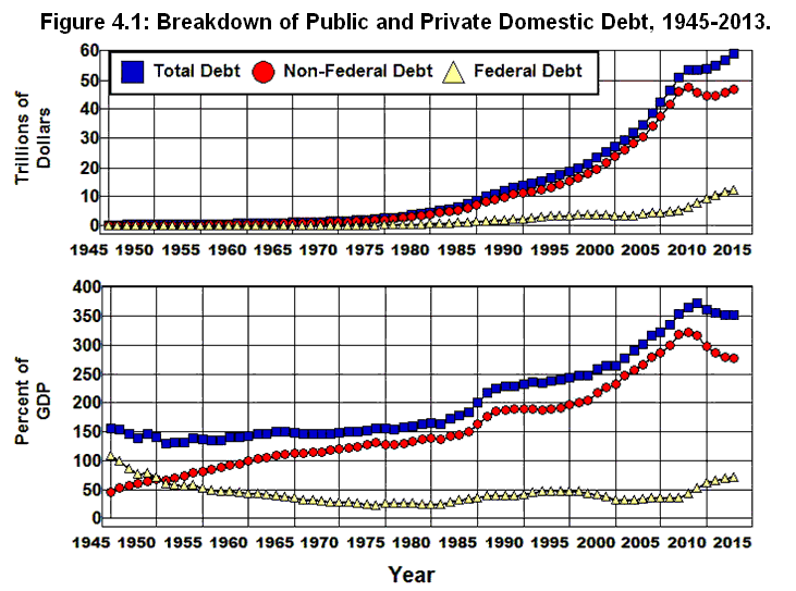
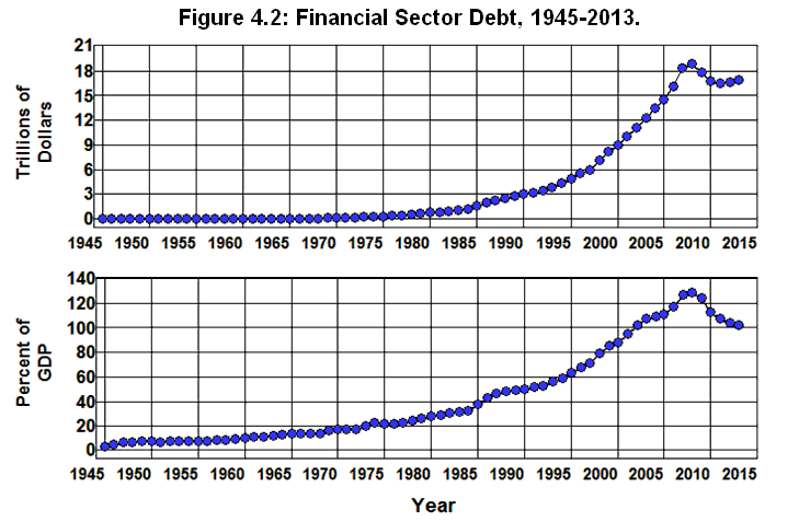
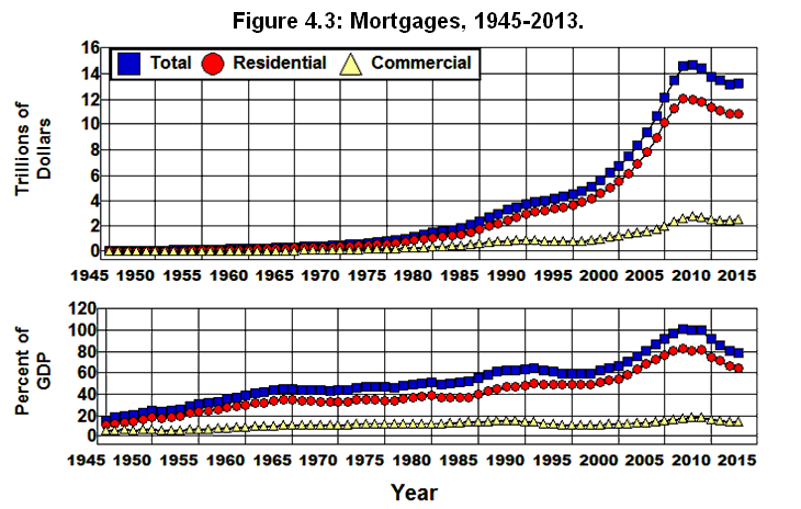
Chapter 5: Nineteenth Century Financial Crises
George H. Blackford © 2009, last updated 5/1/2014
Prior to the Civil War, all you needed to start a bank was a charter from a state and access to a printing press. Banks would accept deposits, make loans, and print banknotes that were, in essence, a promise by the bank to pay the bearer on demand an amount of gold or silver at a fixed price. Banks accepted deposits in the form of gold, silver, and banknotes issued by private banks and made loans, generally in the form of banknotes that they printed themselves. The banknotes printed and issued by private banks circulated in the community alongside coins minted by the United States Mint and the mints of other countries. Given the lack of specie (i.e., gold or silver coins) banknotes printed and issued by private banks served as the primary medium of exchange in the economy and were the dominant form of money.
There was a great deal of financial instability caused by this kind of monetary system, and there were at least three major financial crises prior to the Civil War, one in 1819, 1837, and 1857. At the same time, there were two attempts by the federal government to regulate the financial system during this period. The first was by way of the First Bank of the United States which existed from 1791 to 1811, and the second was by way of the Second Bank of the United States which existed from 1816 to 1836.
First and Second Banks of the U. S.
The First and Second Banks of the United States were the only banks chartered by the federal government prior to the Civil War, and by virtue of the fact that federal deposits were kept in these banks they dominated the financial system. They preformed many of the functions of a central bank in that they policed the other banks in the system by collecting their banknotes and presenting them for redemption in gold or silver thereby limiting the ability of the other banks to print money. In so doing they controlled the money supply and credit conditions in the country and added an element of stability to the financial system.
These banks, however, were private banks chartered to serve the interests of their stockholders, not to serve the public good, and it was felt by many that the political and economic power they wielded by virtue of their relationship to the government was abused. The fate of the Second Bank of the United States was sealed when its president, Nicholas Biddle, opposed Andrew Jackson in the 1832 election. A bill to renew its charter was vetoed by Jackson in that year, and the last nail was driven into its coffin in 1833 when Jackson decreed that no more government money would be deposited in the Second Bank of the United States. (Trumbore eNCyclopedia Phillips)
The demise of the Second Bank of the United States left the country with no financial institution that could perform the functions of a central bank, but even with the First and Second Banks of the United States the situation was far from satisfactory. Since each bank was responsible for the bank notes it issued, one had to evaluate the worth of a given banknote on the basis of the soundness of the issuing bank—that is, its ability to honor its promise to redeem its banknotes in gold or silver—and with hundreds of banks issuing these notes this was no easy task. There were literally thousands of different kinds of banknotes in circulation by 1860, and, as a result, banknotes did not necessarily trade at par. (Dwyer) Banknotes issued by failed banks circulated alongside the notes of sound banks and, of course, counterfeiting has always been a problem—even before the Civil War. (OCC) The result was a very unstable and inefficient monetary system that hindered the growth of trade and economic development. (Grossman)
National Banking Acts of 1863 and 1864
This situation changed dramatically with the passage of the National Banking Acts of 1863 and 1864. These acts created the National Banking System with the intent of providing a stable and uniform national currency and, not coincidently, to help finance the Civil War. These two goals were accomplished by requiring that the banknotes printed by national banks be backed by Treasury securities equal to ninety percent of the value of the banknotes printed by national banks. These securities could then be sold to redeem the notes if the issuing bank failed. In addition, in 1865 a 10% tax was levied on non-national-bank banknotes and on all transactions using non-national-bank banknotes. The existence of this tax essentially forced all banks that wished to print their own banknotes to join the National Banking System.
The fact that banks were forced to purchase Treasury securities in order to print banknotes not only helped to finance the Civil war, it also limited the amount of banknotes that could be circulated in the economic system by the amount of Treasury securities that were available to banks to back the notes they issued. The result was a stable, uniform national currency made up of 1) national banknotes tied to the total value of Treasury debt outstanding, 2) United Sates Notes which were the greenbacks printed by the federal government to pay the troops during the Civil War, and 3) Gold Certificates issued by the Treasury which were, in effect, warehouse receipts for gold held at the Treasury. (OCC)
While the National Banking Acts of 1863 and 1864, bolstered by the 1865 tax on non-national-bank banknotes, did provide a stable and uniform national currency, these dramatic changes in our financial system did not solve the problem of financial crises. The reason is that these reforms failed to deal directly with the fundamental liquidity and solvency problems faced by banks that causes the financial system to be inherently unstable.
Liquidity Problem of Banks
Most businesses can meet their liquidity needs (i.e., their needs for cash) by structuring the term to maturity of their liabilities (i.e., debts that they owe) to match the term to maturity of their assets (i.e., things that they own). They can, for example, finance real estate which yields a return over a relatively long period of time with 15 to 20 year loans, equipment with a shorter lifespan with 5 to 10 year loans, and inventories with loans that corresponds to the period of time it takes for their inventories to turn over. A business that has its liabilities structured in this way can generally muddle through with the hope of rebuilding its equity, even if it is insolvent (i.e., even if it owes more than the value of the assets it can sell to pay its debts) so long as it can service its debt and so long as it can retain the confidence of its short-term creditors.
The situation is fundamentally different for a bank. The primary source of funds for a bank is the deposits it issues, most of which are very short-term liabilities. At the same time most of the assets of the bank are made up of relatively long-term commercial, business, and real estate loans that it makes to its customers. These assets have term to maturities far beyond the term to maturities of the bank's deposits, many of which, namely, checking accounts, are payable on demand. Thus, by their very nature banks are not able to structure the term to maturity of their liabilities to match the term to maturity of their assets.
As was indicated above, an ordinary business can generally muddle through when it is in financial difficulty so long as it can service its debt and retain the confidence of its short-term creditors. This is so because, in general, a relatively small portion of an ordinary business's total liabilities are short term and the number of short-term creditors with which it must contend is relatively small. As a result, an ordinary business generally has the option of sitting down with its local banker and suppliers, opening its books, and undertaking a rational discussion of its financial viability to arrive at a rational decision as to whether or not its short-term credit should be continued. The situation is much different for a bank.
Even a small bank has literally thousands of short-term creditors that hold its deposits, and unlike the debts of most businesses, a large portion of a bank's deposits (its checking accounts) are payable on demand. What’s more, in an unregulated financial system that lacks deposit insurance there is no incentive at all for the depositors of a bank to even listen if a bank tries to explain its financial situation. The depositors know that if the bank were to fail those who close their accounts first while the bank still has cash on hand to cover its withdrawals will not lose their money, while those who wait will not be able to get their money out of the bank until its assets are liquidated. As a result, those who wait potentially risk losing everything.
This means that each individual bank, as well as the entire banking system itself, depends crucially on the confidence the public has in the bank and the banking system. As a result, banks are particularly susceptible to a panic that results in what is known as a run on the bank where all of its depositors lose confidence in the bank and try to close their accounts at the same time. And when a run occurs even the strongest bank can be driven out of business if it is unable to borrow enough funds to meet the demands of its depositors for cash or sell off its assets at prices sufficient to maintain its solvency.
Solvency Problem of Banks
The solvency problem faced by any businesses, including a bank, is best understood in terms of the fundamental equation of double entry bookkeeping:
assets = liabilities + owners' equity
where assets refers to the value of everything the business owns; liabilities refers to the value of everything the business owes, and owners' equity (also referred to as equity, equity capital, or just capital) is defined as the difference between the value of the assets owned by the business and the value of the liabilities owed by the business:
owners' equity ≡ assets - liabilities.
The significance of this equation for our purposes is that it illustrates the solvency problem of banks, namely, the need to maintain a positive owners' equity. If the value of the liabilities of a bank are greater than the value of its assets, its owners' equity (net worth, equity, . . . , etc.) will be negative and the bank will be insolvent. The fact that it is insolvent means that if the bank (or any business that is insolvent) is forced into bankruptcy the value of its assets are insufficient to cover the value of its liabilities and some of its debtors will not get paid back what they have lent to the bank (or business). This is a very precarious situation for a bank because in an unregulated banking system without deposit insurance, no one wants to hold deposits in a bank that is insolvent.
Not only is the liquidity problem of banks fundamentally different from the liquidity problem of ordinary businesses, the solvency problem of banks is fundamentally different as well. Compared to banks, most businesses borrow very little relative to their equity capital, that is, relative to the amount of money the owners of the business have invested in the business. In fact, many businesses operate without borrowing any money at all, and even more borrow less than the amount the owners have personally invested.
The reason for this is that running a business is a risky endeavor. Creditors refuse to lend to a business if the owners do not have a substantial amount of their own money invested in it, and the rates of interest businesses have to pay, especially small businesses, are generally fairly high. As a result, business owners often find it more profitable to reinvest their profits in their business by paying off their debts as soon as possible than to continue to borrow, and the leverage ratio of most businesses—that is, their total debt divided by their equity capital—is relatively small. [5.1]
The situation is much different for a bank. As was noted in Chapter 4, banks are in the business of borrowing from one group of people and lending to another group of people. That's what banks do. They make a profit from the difference between the costs of the funds they borrow in the form of deposits (and during the Nineteenth Century in the form of the banknotes they printed as well) and the revenues they receive from the loans they make to businesses and private individuals. So long as the costs of the funds they borrow are less than the revenues they receive from their loans they can increase their profits by both borrowing and lending more money. What's more, something magical happens when banks lend money.
If you have $1,000 in cash and decide to become a bank, when you lend your $1,000 to someone the chances are that whoever borrowed the money is going to spend it. When the $1,000 you lent is spent the person who receives the money in exchange for whatever is purchased now has your $1,000. He or she has but three choices as to what to do with it: spend it, just hold on to it, or redeposit it in a bank. If the choice is to redeposit it in your bank that means you are able to borrow your $1,000 back from the person who deposits it. As a result your deposits will increase by $1,000 and you get the cash back.
Even if your $1,000 is redeposited in another bank, whatever bank it is redeposited in will be able to borrow your $1,000 back from the person who deposits it and will be able to increase its cash by the $1,000 that you lent. Thus, even though you lose the cash, some other bank will eventually gains the cash unless the non-bank public decides to hold more cash outside the banking system and the cash is not redeposited in a bank.
This is where the magic comes in because what this means is that whenever a bank makes a loan to one of its customers, unless the non-bank public decides to hold all of the newly lent cash outside the banking system, the banking system as a whole does not lose all of the cash that was lent: To the extent it is redeposited in the bank that made the loan that bank gets some of the cash back, and to the extent it is redeposited in some other bank that bank gets some of the cash. In either case the amount of cash in the banking system as a whole does not fall by the amount of the loan.
What does change is the amount of money that the banking system is able to borrow from its depositors. This amount increases by the portion of the loan that is redeposited in the banking system as deposits in the system increase by this amount. In other words, unless the non-bank public decides to hold all of the newly lent cash outside the banking system, whenever a bank makes a loan it increases the amount of money the banking system as a whole is able to borrow from the non-bank public by the amount of the loan that is redeposited in the banking system. No other industry can increase the amount of money it can borrow by increasing the amount of money it lends. It's magic!
The fact that the banking system increases the amount it can borrow when it increases the amount it lends has very important implications with regard to the stability of the financial system. If you were the only bank in a small town during the nineteenth century when you started your bank with $1,000 to lend, and if every time you made a loan all of the proceeds of that loan were subsequently redeposited in your bank, your deposits would grow to $10,000 after you had made ten $1,000 loans while your cash and equity capital would remain at $1,000.
If we ignore the other assets and liabilities of your bank, your financial position would look like Figure 5.1 where your bank’s assets are listed on the left side of the table in this figure, and your liabilities and net worth are listed on the right side of this table.
Figure 5.1: Your Financial Situation after Lending $10,000.
Assets Liabilities & Net Worth Cash Reserves $1,000 Deposits $10,000 Loans $10,000 Net Worth $1,000 Total $11,000 Total $11,000 The fact that your deposits have grown to $10,000 after you have made ten $1,000 loans while your cash and equity remains at $1,000 in this situation means the leverage of your bank (your total debt divided by your net worth) increases from zero when you had no debt in the form of deposits to 10 when your deposits grew to $10,000.[5.2]
This is a very profitable position for you to be in so long as it cost you less to manage your deposits than you make from your loans. If, for example, you can lend at 5% and it cost you 3% to manage your deposits, before your deposits grew you could make only $50 a year by lending out your $1,000 worth of capital. After you lend your $1,000 ten times and your deposits grew to $10,000 you would then be making $200 a year on your $1,000 investment in your bank—you would be taking in $500 on the $10,000 you had lent at 5% and it would cost you $300 (3% of $10,000 worth of deposits) to manage your $10,000 worth of deposits. Thus, instead of only making a 5% return on your $1,000 worth of equity capital you would be making a 20% return on that capital.
Leverage is a beautiful thing for a bank when it comes to making money. If you were able to grow your deposits in this way to $30,000 by making $30,000 worth of loans that were redeposited in your bank, your financial situation would look like Figure 5.2. Your leverage ratio would be 30 to 1, and you would be able to make $600 ($30,000x.05 - $30,000x.03 = $600). This would yield you 60% annual return on your $1,000 investment! Even if it cost you as much as 4% to manage your deposits you would still be able to make $300 in this situation and earn a 30% return on your investment.
Figure 5.2: Your Financial Situation After Lending $30,000.
Assets Liabilities & Net Worth Cash Reserves $1,000 Deposits $30,000 Loans $30,000 Net Worth $1,000 Total $31,000 Total $31,000 While leverage can be a money making machine for banks, it also poses two serious risks. The first comes from the fact that the use of leverage increases the liquidity problem of banks. In the above example, you are only able to achieve 30 to 1 leverage because people are willing to lend you money by depositing it in your bank. You have borrowed $30,000 from your depositors but only have $1,000 worth of cash on hand as a reserve to meet the needs of your depositors for currency. If your depositors take currency out of their deposits faster than you take in currency from the repayment of your $30,000 worth of loans, your reserves of cash will fall. Unless you can find an alternative way to raise cash in this situation—say, by borrowing from other banks or selling some of the asset you own for cash—you are going to be in trouble when you run out of cash since your depositors tend to get upset if you don't have the cash when they try to withdraw money from their accounts.
The second risk comes from the fact that the use of leverage increases your risk of becoming insolvent. If your bank is leveraged at 30 to 1, a 3.3% fall in the value of your assets—say, because some of your debtors go bankrupt or abscond with the money—would wipe out your entire equity because when your equity is leveraged 30 to 1 the value of your equity is less than 3.3% of the value of your assets. The value of your assets would fall below the value of your liabilities, in this situation, and you would then be insolvent. As was noted above, in an unregulated banking system with no deposit insurance no one wants to keep money in an insolvent bank. Even a rumor of your bank's insolvency could start a run and drive you out of business irrespective of your cash reserves or solvency before the run began, and, in the face of a run, as soon as you run out of cash you will be forced to close your doors.
It should be noted that the liquidity and solvency problems of banks are distinct problems. The liquidity problem has to do with having enough cash on hand to meet your day to day obligations. The solvency problem has to do with having assets of sufficient value to cover your debts. If in the above example your debtors absconded with 3.4% your loans, your financial situation would look like Figure 5.3. Your loans would now be worth only $28,980 (.966x$30,000) which means that when we add this to your $1,000 worth of cash the value of your assets would be $29,980 while your liabilities in the form of deposits would be $30,000. You would be insolvent because your liabilities exceed your assets by $20, and you would not be able to pay off all of your depositors if you were forced into bankruptcy even though you still have $1,000 in cash to service your deposits.
Figure 5.3: Your Financial Situation after a 3.4% Loss.
Assets Liabilities & Net Worth Cash Reserves $1,000 Deposits $30,000 Loans $28,980 Net Worth $1,000 Total $29,980 Total $29,980 By the same token, if your debtors had not absconded but instead your depositors decided to withdraw $1,000 from their accounts you would be in trouble even though your solvency hadn't changed. In this situation, your financial situation would look like Figure 5.4. You would still have $30,000 worth of loans even though you lost all of your cash, but since you now have only $29,000 worth of debts in the form of deposits this leaves you with the same net worth of $1,000 that you had before your deposits and cash fell by $1,000. But you would have no cash on hand to meet the demands of your depositors. If someone tries to take money out of their deposit you don't have the cash to give to them even though you still have $1,000 in net worth.
Figure 5.4: Your Financial Situation after a $1,000 Withdrawal.
Assets Liabilities & Net Worth Cash Reserves $0 Deposits $29,000 Loans $30,000 Net Worth $1,000 Total $30,000 Total $30,000 Finally, it should be noted that the ability of banks to increase the amount they can borrow by increasing the amount they lend is not unlimited. It depends crucially on the willingness of the non-bank public to keep their cash in banks. An expansion of bank loans is generally accompanied by an increase in economic activity that increases the need for the non-bank public to hold currency outside of banks to finance their day to day transactions. As a result, it is unlikely that all of the money lent will be redeposited in a bank.
If, for example, you started your small town bank with $1,000 cash and only 96% of your loans were redeposited in your bank you would not be able to leverage you capital 30 to 1 since 4% of the cash you lent would remain outside your bank as the currency held by the non-bank public increased. Thus, by the time you made $25,000 worth of loans your deposits would have increased by $24,000, and you would be out of cash. Your financial situation would look like Figure 5.5.
Figure 5.5: Your Financial Situation with a 96% Redeposit Rate.
Assets Liabilities & Net Worth Cash Reserves $0 Deposits $24,000 Loans $25,000 Net Worth $1,000 Total $25,000 Total $25,000 At this point you would have no more cash to lend. Thus, the maximum leverage you could obtain would be 24 to 1 in this situation, but even this is not obtainable. If you did leverage yourself this far you would have no cash reserves to meet the demands of your depositors in the event one of them wished to make a withdrawal. To play it safe you would have to keep some cash on hand to meet this contingency.
If you chose to keep cash reserves equal to, say, 5% of your deposits to protect yourself from unexpected withdrawals you could then only lend $11,364 before your deposits rose to $10,909 and your cash fell by $455 (4% of your $11,364 worth of loans) to $545 (5% of your $10,909 worth of deposits). At that point your financial situation would look like Figure 5.6.
Figure 5.6: Your Financial Situation with a 96% Redeposit Rate and 5% Reserves.
Assets
Liabilities & Net Worth
Cash Reserves
$545
Deposits
$10,909
Loans
$11,364
Net Worth
$1,000
Total
$11,909
Total
$11,909
You would have to stop lending in order to maintain your cash reserves at 5% of your deposits and would, by choice, be limiting your leverage to a ratio of 10.909 to 1.
Thus, during the nineteenth century the banking business was a continual balancing act between expanding leverage in order to increase profits while maintaining cash and equity reserves to deal with the liquidity and solvency problems that this expansion inevitably entails. This balancing act was made even more difficult by virtue of the fact that when times were prosperous and money was being made hand over fist, the temptation to allow cash reserves to fall and to increase leverage was for many banks irresistible. This was particularly so when people had confidence in the banking system and kept their money in the banks.
Since, in this situation, deposits expand automatically as banks expand their loans, banks automatically receive the cash they need to further expand their loans and, hence, their leverage. If banks did not make a determined effort to expand their cash and equity as their deposits were expanding during prosperous times their cash reserves as a percentage of their deposits would automatically fall and their leverage would automatically increase as well. It is not until the crisis came and the non-bank public lost confidence in the system and began to withdraw their cash that banks would be forced to face the inevitable liquidity and solvency problems they had created for themselves.
Failings of the National Banking System
By virtue of the term structure of their assets and liabilities—that is, the fact that banks borrow short term and lend long term—and the ease with which banks can expand their leverage during prosperous times, the financial stability of banks is much more tenuous than that of an ordinary business. Unfortunately, there was no mechanism within the National Banking System to deal with the tenuous nature of the financial stability of banks. As a result, even though the National Banking System was able to provide a sound and stable currency, it was unable to provide a sound and stable financial system.
One of the reasons for this failing was that there were only two options available to a bank within this system when it needed cash to meet the demands of its depositors: It could either borrow cash from other institutions or to sell whatever asset it owned that it could find a market for. While an individual bank could obtain cash in this way, when the non-bank public wished to increase the currency held outside the banking system, an individual bank could only obtaining the cash in this way either by borrowing from some other bank or by selling something to someone who paid with cash drawn from a deposit in some other bank. There was no mechanism within the National Banking System by which the banking system as a whole could increase the amount of cash available to the system in a situation where the non-bank public wished to increase the amount of cash it held outside the banking system. This led to a serious problem.
During the normal course of economic activity there were seasonal changes in the demand for currency on the part of the non-bank public. When the demand for currency increased, say during the spring when crops were planted and especially during the fall when additional currency was needed to pay seasonal workers during the harvest and to purchase the crops from farmers, currency would flow out of the banks. This would place a strain on the cash available to banks to meet the needs of their depositors and would cause a tightening of the market for bank loans as banks were forced to pay out cash to their depositors as their customers paid off their loans rather than being able to relend the cash they received in this way.
As currency flowed out of the banks to meet seasonal demands, banks were forced to cut back on their loans and interest rates would rise. The pressure on the banks for cash would thus be transmitted to those who relied on the banks for credit. Potential borrowers who were unable to get new loans and debtors who were unable to renew their existing loans at acceptable rates of interest would be forced to cut back their economic activity. At the same time, debtors who could not renew their existing loans would be forced to sell the collateral underlying these loans or to sell other assets they owned in order to meet their obligations to the banks. These forced sales of assets, in turn, caused a general fall in asset prices throughout the system which strained the system even further as debtors found it more difficult to meet their obligations to the banks in the face of falling asset prices. If this strain became particularly severe it would cause some debtors to default which would threaten the solvency of their banks and in some instances lead to bank failures.
Bank failures inevitably shook the confidence of the public and created the possibility of a financial crisis through a run on the system. Once a run began, there was no mechanism within the National Banking System by which it could be contained since there was no way to replenish the cash that a panicked public took out of the banks. When a bank ran out of cash it would be forced to shut down whether it was solvent or not, and if the panic was sufficiently widespread the system would simply implode as the entire system was forced to suspend payments of cash to depositors. The end result was a massive disruption in economic output and employment with extreme hardship throughout the country.
The instability caused by the rigidity of the supply of currency within the National Banking System became clear as the nineteenth century wore on and the country went through the financial crises of 1873, 1893, and 1907. The experiences of these crises eventually led to the creation of the Federal Reserve System in 1913.
Endnote
Leverage is sometimes defined as the ratio of total assets (rather than total debt) divided by equity. Since the fundament equation of double entry bookkeeping (E = A - L) implies that the assets over equity ratio (A/E = L/E + 1) is always one greater than the liabilities over equity ratio, the two ratios measure the same thing, and the choice between them is, for the most part, arbitrary.
[5.2] I have simplified this example of a nineteenth century bank by ignoring the way in which banknotes printed by the bank fit into the operation of the bank and the role played by gold in a banking system encumbered by the rules of the gold standard that existed at the time. These are important to a faithful understanding of how the nineteenth century banking system functioned, but they are ignored here to simplify the exposition in order to highlight those aspects of the nineteenth century system that pertain directly to our modern system.
Chapter 6: The Federal Reserve and Financial Regulation
George H. Blackford © 2009, last updated 5/1/2014
The Federal Reserve System (commonly referred to as "the Fed") was created in response to the crisis of 1907 in an attempt to deal with what was perceived at the time to be the central problem of the National Banking System, namely, the inability of this system to deal with seasonal changes in the demand for currency without placing a strain on banks and their ability to make loans. This problem was dealt with by creating the Federal Reserve System as a central bank—that is, a bank in which other banks can open deposits and from which other banks can borrow money—and by giving the Federal Reserve the power to print its own currency. At the same time, all other banks were prohibited from printing currency. (Bernanke)
The Federal Reserve thus became the lender of last resort within the banking system, willing and—given its ability to print money—able to lend cash to other banks to meet their needs. It was believed that in addition to the ability to meet the seasonal needs of banks for cash, the Fed would also be able to eliminate financial crises by lending cash to sound banks during times of financial stress while allowing unsound banks to go out of business in an orderly fashion.
The mechanism by which the Federal Reserve functions within the financial system, and by which the Federal Reserve derives its power, is quite simple in principle and can be summarized as follows:
The Federal Reserve determines the amount of currency that is available to the economy.
The Federal Reserve also sets the reserve requirement ratio, that is, the fraction of deposits that banks must hold in the form of reserves, where reserves consist of either the currency banks have in their vaults (vault cash) or in their deposit at the Federal Reserve.
The non-bank public is free to determine how much of the currency that the Federal Reserve makes available to the economy is held outside of banks and how much is deposited in banks to serve as reserves against deposits.
Banks are then allowed to expand their loans and deposits (in the manner explained in Chapter 5) until they cannot make additional loans without violating their reserve requirements.[6.1]
Within this system, banks are limited in their ability to expand the amount they can borrow from their depositors as they expand the amount they lend by 1) the amount of currency the Fed makes available to the economic system, 2) the amount of this currency the non-bank public is willing to leave in banks, and 3) the reserve requirement ratio set by the Fed. As is demonstrated below, the cornerstone of this system is the Federal Reserve’s ability to determine the amount of currency that is available to the economic system.
Controlling the Amount of Currency
The amount of currency that is available to the economic system is referred to as high-powered money, where High-Powered Money is the sum of currency in circulation (that is, currency in the hands of the non-bank public) plus the reserves held by banks, either in the form of vault cash or as deposits at the Federal Reserve. High-Powered Money is also referred to as the monetary base as it is the foundation on which the monetary system, indeed, the entire financial system rests.
There are two ways in which the Federal Reserve can control the amount of High-Powered Money, hence, the amount of currency available to society.
The Discount Window
The first is by making or retiring loans to banks. The Federal Reserve makes and retires loans to banks through what is referred to as the discount window where the rate of interest charged for these loans is referred to as the discount rate. All loans made by the Federal Reserve through the discount window must be fully backed by collateral supplied by the borrowing banks, and these loans are made at a discount to the face value of the collateral offered by the borrowing bank. Hence, the terms discount window and discount rate. (FRB)
When the Federal Reserve makes a loan to a bank it does so by simply crediting the reserve deposit of that bank at the Federal Reserve by the amount of the loan. As a result, the reserve component of High-Powered Money is increased directly by the amount of the loan. By the same token, when the Federal Reserve retires a loan previously made to a bank, the bank pays off that loan by deducting the amount of the loan from its reserve deposit at the Federal Reserve. As a result, the reserve component of High-Powered Money is decreased directly by the amount of the loan that is repaid.
The way in which a $1,000 loan by the Fed to a commercial bank affects the financial situation of both the Fed and the Banking system and, thus, changes the amount of currency available to the economic system is illustrated in Figure 6.1. When the Fed credits the amount of this loan to the reserve deposit of the borrowing bank, this transaction increases the Fed’s asset Loans to Banks and its liability Reserve Deposits held by banks by the amount of the loan, $1,000. At the same time, it increases the banking system’s asset Reserve Deposits and its liability Loans from Fed by the same amount.
Figure 6.1: A $1,000 Loan by the Fed to a Bank.
Federal Reserve
Assets
Liabilities
Loans to Banks
+$1,000
Reserve Deposits
+$1,000
Commercial Banks
Assets
Liabilities
Reserve Deposits
+$1,000
Bank Deposits
+$10,000
The fact that the reserve deposits in the banking system have increased by $1,000 as a result of this loan means that High-Powered Money—the sum of currency in circulation and reserve deposits—has increased by this amount, and since banks can withdraw an additional $1,000 worth of currency from their reserve account at the Federal Reserve after this transaction it means that the amount of currency available to the system has increased by $1,000.
This process, of course, works in reverse when the loan is paid back by the bank. The Fed’s asset Loans to Banks and its liability Reserve Deposits will fall by the amount of the repayment as the bank repays the loan by allowing the Fed to deduct the amount of the repayment from the bank's reserve deposit. At the same time, the banking system’s asset Reserve Deposits and its liability Loans from Fed will fall by the same amount. Thus, all of the pluses in Figure 6.1 become minuses.
The fact that the reserves in the banking system must decrease by the amount of the repayment means that High-Powered Money will fall by this amount as well, and there will be $1,000 less currency available to the economic system than there was before the repayment took place since banks will now be able to withdraw $1,000 less currency from their reserve accounts than they could before the loan was made.
Open Market Operations
The second way in which the Federal Reserve can control the amount of High-Powered Money is by buying or selling something. While it doesn’t matter what the Federal Reserve buys or sells, when it comes to controlling the amount of High-Powered Money the Federal Reserve generally restricts itself to buying or selling government securities. The decisions of the Fed to buy or sell government securities are made by the Federal Reserve’s Open Market Committee and are referred to as the Federal Reserve’s open market operations. (FRB)
When the Federal Reserve buys a government security, the institution that sells the security receives a check written on the Federal Reserve for the amount paid for the security. In the normal course of events, the check will be deposited in a bank, and, in turn, the bank will redeposit the check in its reserve account at the Federal Reserve. As a result, the reserve component of High-Powered Money will increase by the amount of the check written on the Federal Reserve to purchase the government security.
Figure 6.2 illustrates the situation where the Fed purchases a $1,000 government security from a member of the non-bank public. This transaction increases the Fed’s asset Government Securities by the amount of the purchase, $1,000. When the member of the non-bank public deposits the check it received for the security in its bank account, the banking system’s liability Bank Deposits increase by the amount of the check. When the bank deposits the $1,000 check in its reserve account the banking system’s asset Reserves increases by the same amount as will the Fed's liability Reserve Deposits.
Figure 6.2: A $1,000 Purchase of Government Security by the Fed.
Federal Reserve
Assets
Liabilities
Gov. Securities
+$1,000
Reserve Deposits
+$1,000
Commercial Banks
Assets
Liabilities
Reserve Deposits
+$1,000
Bank Deposits
+$1,000
Non-Bank Public
Assets
Liabilities
Bank Deposits
+$1,000
Bank Loans
+$1,000
Gov. Securities
-$1,000
The only change that has occurred in the financial situation of the non-bank public at this point is there has been an exchange of one kind of asset for another—Government Securities held by the non-bank public have gone down while Bank Deposits held by the non-bank public have gone up by the same amount, $1,000. But the fact that the reserves in the banking system have increased by $1,000 as a result of this purchase by the Fed means that High-Powered Money has increased by this amount, and there is now $1,000 more currency available to the economic system than there was before this purchase took place.
By the same token, when the Federal Reserve sells a government security it will receive a check written on a commercial bank for the amount of the sale. The Federal Reserve will then deduct the amount of that check from the reserve deposit of the bank on which the check is written, and the reserve component of High-Powered Money will decrease by the amount of the check. The bank, in turn, will deduct the amount of the check from the account on which the check was written. As a result, all of the signs in Figure 6.2 will be reversed, and the amount of High-Powered Money, that is, the amount of currency available to the economic system, will be decreased accordingly.
Thus, when the Fed wants to increase the amount of currency available to the economy it can either increase the amount it lends to banks or it can purchase government securities. When the Fed wants to decrease the amount of currency available to the economy it can either reduce the amount it lends to banks or it can sell government securities.
Seasonal Demand for Currency
The ability of the Federal Reserve to control the amount of currency that is available to the economic system provided a mechanism by which the seasonal demand for currency problem that plagued the National Banking System could be eliminated. After the Federal Reserve came into being, banks were no longer forced to contract their lending as currency flowed out of the banks in response to seasonal changes in the demand for currency. Instead they could borrow from the Fed or the Fed could purchase government securities from the public in order to replenish the reserves that were lost as the currency flowed out of the banks, for example, during spring planting or the fall harvest. By the same token, when the planting or harvest was over and the currency flowed back into the banks the Fed could absorb the excess currency as the loans it had made were repaid and as it sold the government securities it had purchased to meet the currency drain from banks during the planting or harvest seasons.
It is important to note, however, that when the Federal Reserve changes the amount of High-Powered Money in this way it can lead to changes in the financial system that go beyond the changes indicated in Figure 6.1 and Figure 6.2 above. The Federal Reserve is not simply a passive agent that responds to the seasonal changes in the demand for currency by the non-bank public. The Fed can change the amount of High-Powered Money through its lending and open market operations in any way it chooses whether currency is flowing into or out of banks or not. As a result, the Federal Reserve has the power to affect the ability of the banking system to make loans. This gives the Federal Reserve the power to affect the credit conditions in the economic system irrespective of the seasonal demands for currency by the non-bank public.
Controlling Loans and Deposits
Consider the situation depicted in Figure 6.2 where the Fed has purchased a $1,000 government security from a member of the non-bank public and thereby increased the amount of deposits and reserves in the banking system by $1,000. Now assume that the reserve requirement ratio is 10% and the banking system is fully loaned up before this transaction takes place—that is, that the actual reserves held by banks are equal to the reserves they are required to hold as determined by the size of their deposits and the reserve requirement ratio.
Since the reserve requirement ratio is 10% and this transaction increased deposits by $1,000 the reserves banks are required to hold have increase by $100. At the same time, this transaction also increases the reserves that banks actually have by $1,000. As a result, there is $900 in excess reserves in the banking system ($1,000 increase in actual reserves minus the $100 increase in required reserves) after this transaction takes place that did not exist before this transaction took place. These excess reserves represent cash banks hold in excess of what they are required to hold—cash that can be lent to and borrowed back from the non-bank public as loans and deposits grow in the banking system in manner discussed in Chapter 5.
As banks make loans to and borrow the money back from the non-bank public the loans and deposits in the banking system can grow until there are no longer excess reserves in the banking system. If there are no leakages of currency out of the banking system as this process of expansion takes place, the system will eventually reach the point depicted in Figure 6.3 where Bank Deposits increase by $10,000 and bank loans by an additional $9,000.
Figure 6.3: Secondary Effects of a $1,000 Purchase by the Fed.
Federal Reserve
Assets
Liabilities
Gov. Securities
+$1,000
Reserve Deposits
+$1,000
Commercial Banks
Assets
Liabilities
Reserve Deposits
+$1,000
Bank Deposits
+$10,000
Bank Loans
+$9,000
Non-Bank Public
Assets
Liabilities
Bank Deposits
+$10,000
Bank Loans
+$10,000
Gov. Securities
-$1,000
At this point the process of expansion must come to an end as required reserves will have increased by $1,000 (10% of the $10,000 increase in deposits), and there will no longer be excess reserves in the system. At the same time, the non-bank public will have increased the deposits it owns by an additional $9,000 and will have gone $9,000 deeper in debt to the banks. And all of this has taken place as a result of 1) the Federal Reserve purchasing a $1,000 government Security, 2) the banking systems willingness to lend its excess reserves, and 3) the non-bank public's willingness to deposit its excess cash in banking system.
This process works in reverse, of course, if the Federal Reserve sells a $1,000 government security. Reserves and deposits would fall by $1,000, and banks would find themselves with a $900 deficiency in reserves. Banks would then be forced to reduce their outstanding loans by $9,000 as the non-bank public paid off their debts to the banks and bank deposits would fall by an additional $9,000. All of the signs in Figure 6.3 would be reversed and there would no longer be a deficiency of reserves in the system.
The same kinds of results would be obtained if the Federal Reserve had increased its loans to banks by $1,000 in this situation instead of purchasing a government security. The only difference would be that the loan would not have directly increased deposits by $1,000, and the non-bank public would not have sold a government security. The entire $1,000 increase in reserves would be excess reserve, and banks would be able to increase their loans to the non-bank public by $10,000 instead of only $9,000. The end result would be as depicted in Figure 6.4.
Figure 6.4: Secondary Effects of a $1,000 Loan by the Fed.
Federal Reserve
Assets
Liabilities
Loans to Banks
+$1,000
Reserve Deposits
+$1,000
Commercial Banks
Assets
Liabilities
Reserve Deposits
+$1,000
Bank Deposits
+$10,000
Bank Loans
+$10,000
Loans from Fed +$1,000
Non-Bank Public
Assets
Liabilities
Bank Deposits
+$10,000
Bank Loans
+$10,000
Again, if the Fed had reduced its loans to banks by $1,000 instead of increased its loans by this amount all of the signs in Figure 6.4 would be reversed.
Roaring Twenties and Great Depression
While the Federal Reserve was able to solve the seasonal demand for currency problem that had plagued the National Banking System, it was not able to solve the financial crisis problem that it was hoped it would solve. The inadequacy of the Federal Reserve in this regard became painfully obvious as the economy worked its way through the Roaring Twenties and into the Great Depression of the 1930s.
As was noted in Chapter 4, the 1920s began with a minor recession in 1920-21, and then a speculative bubble in the real estate market began in 1921 and burst in 1926. (White) This real estate bubble was superseded by a speculative bubble in the stock market which began in 1926 and burst in October of 1929. As real estate and stock prices fell the economy went into a recession, asset prices fell, debtors defaulted on their loans, and a banking crisis began in the fall of 1930 that didn't reach its climax until 1933 when some 5,190 banks went under in that year alone.
As this drama unfolded it became impossible for the Federal Reserve to resolve the situation by simply providing cash to sound banks in order to save them while allowing unsound banks to go under. Even though the Fed was able to deal with the liquidity problems of banks in meeting the demands of their depositors during the crisis, it was powerless when it came to dealing with the solvency problems of banks that developed during the crisis. The problem was not that sound banks needed cash to meet their depositor’s demands for currency. The problem was that the forced sale of assets throughout the system caused asset prices to fall, which, in turn, caused the value of the collateral underlying bank loans to fall below the value of the loans that had been made. This drove otherwise sound banks into insolvency, and banks became unsound faster than they could be saved. The result was the downward spiral described in Chapter 4 that led to the Great Depression of the 1930s. (Fisher Keynes Kindleberger)
The experience of the 1920s also revealed a number of serious deficiencies in the way the Federal Reserve was organized. Because of the inherent mistrust of government in the United States at the time the Federal Reserve was founded, there was a determined effort to decentralize power within the Federal Reserve System. Toward this end, the Federal Reserve was created as a voluntary, quasi private institution owned by the member banks, that is, by the banks that choose to join the Federal Reserve System. Instead of creating a single bank, the country was broken up into twelve banking districts, each of which was given its own Federal Reserve Bank. Each Federal Reserve Bank was governed by a nine member board of directors, six of which were elected by the member banks in its district and the remaining three were appointed by a seven member Federal Reserve Board that was established to oversee the system as a whole. The Secretary of the Treasury and Comptroller of the Currency served on the Federal Reserve Board ex officio and the remaining five members were appointed by the President and confirmed by the Senate. This arrangement insured that the individual Federal Reserve banks would be dominated by the member banks rather than by the federal government.
In addition, even though the government appointed Federal Reserve Board was established to oversee the system as a whole, the lines of authority and responsibility between the board and the district banks were not clearly drawn. As a result, there was no central authority within the system, and it was impossible for the Federal Reserve to pursue a unified or coherent national policy in the absence of a consensus since each of the twelve Federal Reserve district banks were free to follow their own lending and open market policies irrespective of the policies of the other district banks or those of the Federal Reserve Board. (Meltzer)
To make things worse, there were few provisions in the original Federal Reserve Act that allowed the Federal Reserve to regulate or control the kinds of behavior on the part of financial institutions that inevitably lead to financial crises. The focus of the act was on providing an elastic currency within the context of a decentralized system rather than on regulating or controlling the behavior of financial institutions as such.
All of these factors combined to make it impossible for the Federal Reserve to curb the speculative behavior in the real estate and stock markets that led to the Crash of 1929 and, in fact, made it virtually inevitable that the Fed would finance the increase in debt that occurred during the 1920s that ultimately lead the country through a downward spiral of defaults and into the Great Depression of the 1930s. (Fisher Keynes Friedman Kindleberger Meltzer Eichengreen Bernanke)
The Curse of Prosperity
The problem of financial crises arises from the very nature of the financial system itself, starting with the fact that the financial system is, by its very nature, inherently unstable. As was explained in Chapter 5, during periods of economic growth and prosperity the temptation to allow cash reserves to fall and to increase leverage is irresistible for many financial institutions. In this situation we find that poorly managed financial institutions, by the very fact that they are poorly managed, tend to underestimate the risks of economic instability as they see the road to riches in increasing their leverage and in financing projects that pay the highest expected rates of return. Those projects inevitably turn out to be the most speculative projects that are the most at risk from economic instability. To make matters worse, as was explained in Chapter 4, there are powerful incentives for financial institutions to finance these projects since huge fortunes can be made by those who facilitate and are able to take advantage of the speculative bubbles that are created by this kind of speculative activity.
In addition, while most people are honest, many are not. In an unregulated or poorly regulated financial system opportunities for fraud abound, and no other sector of the economy has the potential for illicit gains as does the financial sector. (Black Fisher Phillips) It is no accident that the most notorious fraud of all time was perpetrated by Charles Ponzi—the man for whom the Ponzi scheme was named—during the unregulated era of the Roaring Twenties or that the greatest Ponzi scheme of all time was perpetrated by Bernie Madoff during the recent period of deregulation. Nor is it a coincidence that the frauds of Charles Keating, Michael Milken, Ivan Boesky, Jeff Skilling, Ken Lay, Andy Fastow, and Bernie Ebbers occurred during this latter period. As these individuals and countless others have shown, fortunes can be made in the financial sector by people who fraudulently game the system, and this fraud is most dangerous when it involves banks. Given the banking system’s ability to increase the amount it can borrow as it increase the amount it lends and the fact that a substantial portion of the banking system’s liabilities, namely its checking accounts, are payable on demand, the banking system is particularly vulnerable to a run that can bring down the entire system like a house of cards.
This danger is particularly acute during prosperous times when highly leveraged, poorly and fraudulently managed banks can earn more money than moderately leveraged well managed banks. In this situation poorly/fraudulently managed banks can offer higher rates of interest to their depositors. This gives them a short-term competitive advantage in the market for bank deposits. At the same time, this situation presents a dilemma to the well managed banks. If they do not follow the lead of the poorly/fraudulently managed banks by matching the increases in interest on their deposits the well managed banks will lose deposits to poorly/fraudulently managed banks. What's more, if they do match these increases they will lose money unless they also abandon their reluctance to increase their leverage and finance the kinds of riskier speculative projects being financed by the poorly managed banks. (Black Fisher Phillips) As a result, the very existence of the well managed banks is threatened in this situation if they fail to follow the lead of the poorly/fraudulently managed banks.[6.2]
In addition, there are powerful psychological and social pressers that come to bear on those who try to run a well managed bank in this situation. When others are making fortunes through what seem to be unsound competitive practices that threaten your bottom line, it is exceedingly difficult to risk being wrong on your own in standing up and going against the tide. It is much easier to follow the crowd and risk going down together. As was noted by John Maynard Keynes some seventy-five years ago
A sound banker, alas, is not one who foresees danger and avoids it, but one who, when he is ruined, is ruined in a conventional way along with his fellows, so that no one can really blame him. (Keynes)
All of this feeds the speculation that leads to bubbles where prices are bid up to unsustainable levels and then fall precipitously as the markets crash. This situation is similar to the effect on competitors when an ordinary business recklessly cuts prices and bids up the costs of resources, but the analogy ends here because there are two fundamental differences between ordinary businesses and banks.
First, unlike an ordinary business, when a poorly or fraudulently managed bank underestimates the risks of economic instability, leverages itself to dangerous levels, and increases interest rates on its deposits thereby inducing its competitors to follow suit it threatens the stability of the entire financial system. If the bank is a particularly large or important bank, or if a relatively large number of its competitors are driven out of business, it can cause depositors to lose confidence in the system itself, and the ensuing panic can bring down the entire financial system as depositors try to get their money out of the banking system.
Second, no other sector of the economy is as intricately intertwined with the entire economic system as is the financial sector in which banks play a central role. When this sector falters in the wake of a bursting speculative bubble it puts the entire economic system at risk. We don’t have to imagine a situation in which the financial difficulties of banks in an unregulated or poorly regulated financial system can bring down the entire economy. This has proved to be the inevitable result throughout the history of banking and around the entire world whenever a banking system has been caught up in this kind of situation. (Reinhart Rogoff Kindleberger MacKay Skidelsky 1819 1837 1857 1873 1893 1907 Friedman Galbraith)
Reforming the System
In 1932 the Senate Committee on Banking and Currency set out to investigate the cause of the developing depression. This investigation became known as the Pecora Commission after its chief counsel, Ferdinand Pecora. Pecora exposed massive levels of fraud, corruption, conflicts of interest, and incompetence on Wall Street which led to a public outcry for government regulation of the financial sector. (Moyers Galbraith) The result was passage of the Glass-Steagall Act of 1933 which created the Federal Deposit Insurance Corporation (FDIC) and required the separation of commercial from investment banking and insurance to eliminate conflicts of interests that had fostered corruption in the markets for securities. In addition, the Banking Act of 1935 centralized control of the Federal Reserve System in the Federal Reserve Board. (Bernanke) The Federal Reserve Board was also symbolically renamed the Board of Governors of the Federal Reserve System in the Banking Act of 1935, and the Board of Governors was reconstituted as its ex officio members were replace by members appointed by the president and confirmed by the Senate.
At the same time, the legal authority to implement Federal Reserve policy was taken out of the hands of the individual Federal Reserve district banks and vested in a newly created Federal Reserve Open Market Committee (FOMC) made up of the seven members of the Board of Governors and five of the presidents of the individual Federal Reserve district banks. The five presidents serve on a rotating basis except for the president of the New York Federal Reserve Bank who, because of the importance of New York City to the financial system, was given a permanent seat on the FOMC. In addition, the Fed was given enhanced power to regulate and control speculative activities within the financial system. It was given the power to set margin requirements on loans collateralized by shares of stock, for example, and to intervene in other financial markets as the need arose.
The point of this legislation was to provide a comprehensive system of government regulation designed to prevent financial crises before they began. At the heart of this system was the FDIC insurance of bank deposits designed to prevent runs on banks. While deposit insurance may prevent runs it cannot eliminate financial crises because it does nothing to keep poorly or fraudulently managed banks from overextending themselves. Toward this end, the kinds of loans banks were allowed to make were were severely restricted as was the amount of money a bank was allowed to loan to a single customer.
To prevent poorly/fraudulently managed banks from having a competitive advantage over well managed banks in competing for deposits, banks were prohibited from paying interest on demand deposits (i.e., checking accounts), and the maximum interest rates banks were allowed to pay on time deposits (i.e., savings accounts) was set by the Fed. These rules were designed to protect the public and taxpayers (by way of the FDIC) from reckless and fraudulent behavior on the part of banks. And to make all of this work, a comprehensive regulatory and supervisory system was put in place to ensure that banks were following the rules set down by the Fed and not gaming the system to get around the rules.
A similar regulatory system was put in place for thrift institutions such as savings and loan associations via the Federal Home Loan Bank Act of 1932 which created the Federal Home Loan Banking System (FHLB) that regulated savings and loan associations and the National Housing Act of 1934 which created the Federal Savings and Loan Insurance Corporation. (FSLIC)
From the 1930s through the 1960s policy makers took a decidedly pragmatic view of financial regulation in reining in the speculative and fraudulent urges of the financial sector. Haunted by the specter of the Great Depression, they strengthened the regulatory system as the need arose. The Securities Exchange Act of 1934 created the Securities and Exchange Commission (SEC) to regulate investment banks and the stock exchanges in order to crack down on fraud and corruption in the securities markets. Publicly traded corporations were required file disclosure statements with the SEC to make public important information about their firms subject to both civil and criminal penalties for false or misleading statements or for important omissions. Insider trading was also outlawed as were the stock manipulation practices such as front running, disseminating false information, and artificially trading a security to mislead investors.
The Maloney Act of 1938 amended the Securities Exchange Act to create Self Regulating Organizations (SROs) to provide direct oversight of securities firms under the supervision of the SEC and provided for the regulation of the Over-The-Counter (OTC) market for securities. The SEC was also authorized to impose its own capital requirements on securities firms, and in 1944 the SEC exempted from its capital rule any firm whose SRO imposed more comprehensive capital requirements.
In 1940 Congress passed the Investment Company and Investment Advisers Acts which brought mutual funds under the purview of federal regulation, and in 1956 the Bank Holding Company Act was passed restricting the actions of bank holding companies. The International Banking and Financial Institutions Regulatory and Interest Rate Control Acts were passed in 1978 to bring foreign banks within the federal regulatory framework and to establish the limits and reporting requirements for bank insider transactions. (RiskGlossary)
This regulation was designed to break the boom and bust cycle in the financial sector of the economy—which inevitably led to a boom and bust cycle in the economy as a whole—by prohibiting the kinds of reckless and irresponsible speculative and fraudulent practices that inevitably lead to insolvency on the part of poorly and fraudulently managed banks and drove many responsibly managed banks out of business and the system into crises. What's more, these measures actually worked for over fifty years to accomplish this end. Unfortunately, things began to change in the 1970s and 1980s as attitudes toward government regulation of the economic system began to change.
Endnotes
[6.1] While this mechanism is quite simple in principle, it is somewhat more complicated in practice. The Federal Reserve System is a voluntary organization, and not all banks are members of the system. Prior to 1980, the Fed only set the reserve requirement for member banks, that is, for banks that chose to become members of the Federal Reserve System. Reserve requirements for nonmember banks were set by the states in which the nonmember banks were chartered. In addition, there are different reserve requirements for different kinds of deposits, e.g., time deposits (savings accounts) have lower reserve requirement ratios than demand deposits (checking accounts). What's more, the amount of currency banks held in their vaults (i.e., vault cash) was not considered to be part of reserves from 1917 to 1959. To simplify the exposition in what follows these considerations are ignored and it is assumed there is only one reserve requirement ratio that applies to all deposits and that vault cash is part of reserves. See Feinman for a history of the way reserves and reserve requirements were determined from the nineteenth century through the early 1990s.
[6.2] The nature of the problem here was succinctly put by Charles Prince, former CEO of Citigroup, in his infamous and much maligned comment in the Financial Times: "When the music stops, in terms of liquidity, things will be complicated. But as long as the music is playing, you’ve got to get up and dance. We’re still dancing.” (See Reuters)
Chapter 7: Rise of the Shadow Banking System
George H. Blackford © 2009, last updated 5/1/2014
As memories of the Great Depression faded, an antigovernment movement began to take hold in the United States led by a group of people who possessed an abiding faith in the efficacy of free markets to solve all economic problems. This movement became the foundation of the Conservative Movement in the 1960s and, in turn, provided the ideological foundation of the Republican Party in the 1970s. Their mantra of lower taxes, less government, and deregulation combined with disdain for government has dominated the political debate ever since. These ideas were in the forefront of the Reagan Revolution that began with the election of Ronald Reagan in 1980, and, as was noted in Chapter 4, they were embraced by the Democratic Party in the 1990s. They reached a crescendo in the 2000s after the Republican Party took control of both the Whitehouse and Congress in 2000. (Harvey Frank Amy Westen Altemeyer)
The success of the Conservative Movement over the past thirty years in undermining the regulatory framework setup in response to the disaster that followed in the wake of the Crash of 1929 has been phenomenal—not only in passing legislation that deregulated our financial institutions but in reducing the funding for regulatory agencies and in fostering a non-enforcement attitude toward existing regulations as well. At the same time, changes took place in our financial system that made what was left of our regulatory system in the early 2000s essentially unworkable.
Deregulation in the 1980s
It was clear in 1980 that thrift institutions (i.e., savings banks and savings and loan associations) were in serious trouble as a result of the rise of Money Market Mutual Funds (short-term mutual funds with all of the characteristics of a savings account) and Cash Management Accounts (money market funds that allowed customers to withdraw their funds by writing a check) in the 1970s. Even though these funds were uninsured, the high interest rates in the late 1970s caused by the high rate of inflation during that era allowed money market funds to invest directly in Treasury securities backed by the full faith and credit of the federal government as well as in highly rated corporate debt and still pay a higher rate of interest to investors than was available on the regulated accounts at banks. Thus, given the high quality of their investments, money market funds did not have to be insured to compete directly with the insured deposits of banks, and the resulting loss of deposits to money market funds put depository institutions in a serious bind.
At the same time there was a second change in the financial system that was having a negative effect on banks, namely, the development of the market for Repurchase Agreements—a collateralized loan agreement wherein the borrower sells a security to a lender with the understanding that the borrower will buy it back (i.e., repurchase it) on a specific date at a higher price, the difference in price being the interest earned by the seller/lender. (FRBNY FDIC)
The market for repurchase agreements (and money market funds to the extent they invested in short-term corporate debt) competed directly with banks for their short-term loans. This was so because the existence of an efficient market for repurchase agreements gave large depositors at banks the choice of leaving their unused balances in non-interest earning checking accounts or earning a return on these balances by lending them out for short periods of time, even as short as overnight, in the repurchase market. Borrowers in these markets, thus, had a choice of borrowing for short periods of time either from a bank or from its depositors.
By 1980 it was felt that something had to be done about money market funds and repurchase agreements—that either these markets had to be regulated in such a way as to keep them from competing with banks, or banks had to be deregulated. In the deregulatory spirit of the times, this led to passage of the Depository Institutions Deregulation and Monetary Control Act of 1980 (DIDMCA) which authorized Negotiable Order of Withdrawal (NOW) and Automatic Transfer System (ATS) accounts that effectively allowed banks to pay interest on their checking accounts and write checks on their savings accounts. At the same time DIDMCA provided a mechanism by which interest rate ceilings on time deposits (savings accounts and certificates of deposit) would be phased out by 1986, and there was an expansion in the kinds of loans and investments that thrifts were allowed to make. This act also increased the insurance on deposits from $40,000 to $100,000. (FDIC)
While this act allowed banks, in effect, to pay interest on their checking accounts and write checks on their savings accounts, and, thus, to compete with money market accounts for deposits, it left the repurchase agreement market completely unregulated and the money market funds almost so, and it did little to solve the immediate problem of these institutions drawing off funds from banks, especially thrifts. Thrifts held long-term assets, mostly mortgages, that paid fixed rates of interest. They could not increase the interest rates on their deposits to match the rates offered by money market funds without losing money. At the same time, when market rates go up, the value of assets that pay fixed rates of interest go down. Thus, as thrifts lost deposits to money market funds they were forced to sell off their long-term assets at a loss to fund the withdrawals of their depositors.
By 1982 thrifts were in serious trouble as a result of the economic recession and the high interest rates caused by the anti-inflationary policies of the Fed. In response the Garn–St. Germain Depository Institutions Act of 1982 was passed to further deregulate banks. This act lessened the capital and reserve requirements of banks; provided mechanisms to assist failing banks rather than closing them; accelerated the phase out of interest rate ceilings, and further expanded the kinds of loans and investments thrifts could make so as to allow them to become more like commercial banks that were fairing much better in the financial turmoil of the times than were thrifts. (FDIC) It also allowed banks to offer interest-only, balloon-payment, and adjustable-rate (ARM) mortgages. In addition, in the years that followed, the Federal Reserve and the Comptroller of the Currency (the chief regulator of national banks) further relaxed the restrictions on the kinds of loans banks could make and allowed the non-bank subsidiaries of bank holding companies to buy and sell securities, such as derivatives, that they had previously been barred from holding. (FCIC)
It was thought that increasing competition in the financial sector by allowing thrifts to become more like commercial banks and allowing thrifts and commercial banks greater flexibility in competing with mutual funds and in the market for repurchase agreements the system could be made stronger and more efficient. All that was needed to bring this about was stable or declining interest rates to relieve the pressure on the solvency of thrifts. Interest rates did continue to decline as hoped, but, unfortunately, the deregulatory provisions of these two acts in the hands of the free marketeers of the Reagan Administration led to an unmitigated disaster.
The free-market philosophy of Reaganomics called for less government intervention in the market place. The idea was to get the government out of the way and just let the market sort things out as these institutions competed their way out of the problems they were in. The result was a reduction in the budgets and staffs of the regulatory agencies. This led to less examinations and regulatory supervision at these institutions at a time when the thrift institutions were in financial difficulty and attempting to expand their operations into new areas. (FDIC Black)
As was noted in Chapter 1, the result was the savings and loan crisis that began in the late 1980s—the first financial crisis to hit the United States since the Crash of 1929. In the end, some 1,300 savings institutions failed, along with 1,600 banks, a total that, ironically, was greater than the 2,800 institutions newly chartered under the policy that led to this crisis. In addition, some 300 fraudulently run savings and loans that were nothing more than Ponzi schemes failed at the peak of this disaster, over a thousand individuals associated with the savings and loan debacle were convicted of felonies, and it costs the American taxpayer $130 billion to clean up the mess. In addition, this financial crisis was a precursor to the 1990-1991 recession. (Black FDIC Krugman Akerlof Stewart)
The decision to deregulate the banking system in the face of the competition from money market funds and the markets for repurchase agreements in the early 1980s, rather than to expand the regulatory system to bring these funds and markets under the umbrella of the existing regulatory system, had profound effects on the financial system that went far beyond the savings and loan crisis. In understanding these effects it is instructive to review how financial markets are organized and to examine the kinds of instruments that are traded in these markets. It is also necessary to look at the role collateralization plays in today’s financial system.
Financial Markets and Instruments
The financial system is generally broken down into two markets: The capital market which is concerned with long-term financing for periods of more than a year and the money market which is concerned with short-term financing for periods less than a year.
The Capital Market
Stocks, bonds, and mortgages are sold in the capital market where Stocks are certificates of ownership of a corporation that give the holder a say in the management of the corporation and a right to its equity and profits. More simply put, the stock holders are the owners of the corporation.
A bond is a financial instrument that defines the terms on which the issuer—a government or a corporation—agrees to borrow money. A bond generally has 1) a face value that defines how much the issuer (borrower) will pay the holder (lender) when the bond matures, 2) a maturity date that defines when the issuer will pay the holder the face value of the bond, and 3) an amount of interest and the terms, usually quarterly or biannually, on which interest will be paid to the holder of the bond.
Bonds may or may not be backed by collateral. If a bond is backed by collateral it is a collateralized bond and the bondholder has a right to the collateral in the event the issuer defaults, that is, fails to live up to the terms of the bond. If a bond is not backed by collateral it is an uncollateralized bond. In the event of a bankruptcy the holder of an uncollateralized bond has a claim against whatever is left over after the collateralized creditors have claimed their collateral. Stock holders, being the owners of the corporation, are entitled to whatever is left, if anything, after all of the creditors are paid.
A mortgage loan is essentially a collateralized bond where the collateral is real estate owned by the issuer of the mortgage.
The Money Market
There are a number of financial instruments—generally referred as "paper"—that are bought and sold in the money market, the most important being:
Brokered Certificates of Deposit which are fixed term time deposits issued by banks and sold by brokers such as Merrill Lynch.
Repurchase Agreements which are collateralized loan agreements wherein, as was noted above, the borrower sells a security to a lender with the understanding that the borrower will buy it back (i.e., repurchase it) on a specific date at a higher price, the difference in price being the interest earned by the lender. If the borrower defaults the lender can keep or sell the security.
Commercial Paper which are promissory notes (i.e., IOUs) that may or may not be collateralized, issued by corporations with strong credit ratings. If the borrower defaults the lender has a right to the collateral if the paper is collateralized. Otherwise the lender is a lesser creditor in the event of bankruptcy.
Bankers' Acceptances which are a promise of a bank to pay a specified amount of money to the holder at a specified time and are generally used in international trade as a way to guarantee payment by a third party upon delivery;
Treasury Bills which are short-term government bonds with a maturity date less than a year.
Federal Funds which are the borrowing and lending of reserves between banks.
Importance of Collateralization
Before the development of markets for collateralized financial instruments, most long-term financing was obtained in the bond market by issuing uncollateralized bonds or through the mortgage market by obtaining a mortgage loan directly from a bank or an insurance company. By the same token, most short-term financing was obtained by borrowing directly from a bank.
As a result, virtually all financing was obtained in highly regulated markets from lenders who had a powerful incentive to examine carefully the credit worthiness of the borrower. In the case of uncollateralized bonds and unsecured loans, if the borrower defaulted and filed for bankruptcy the lender would get only what was left after the secured creditors claimed their collateral. In the case of mortgage loans, the lender would get the property secured by the mortgage, but there were costs involved, and if the value of the property fell the mortgagee stood to lose. In addition, the SEC, Fed, FDIC, and state banking and insurance agencies provided stability to these markets by overseeing them to prevent, as much as possible, recklessness and fraud on the part of borrowers and lenders.
With the rise of collateralized financial instruments the structure of the financial markets changed—at first gradually in the 1970s and 1980s and then explosively in the 1990s and 2000s.
Before the development of these instruments relatively few borrowers had access to the money market other than through a bank because lenders were unwilling to lend in this market to any but the most credit worthy borrowers. The reason was the lenders in this market were forced to take a close look at the creditworthiness of the borrower before they made a loan since they were unsecured creditors and at risk of a serious loss if the borrower defaulted. Only banks had the kind of personal contact with their borrowers to effectively evaluate the creditworthiness of most borrowers.
When the loan was collateralized the focus shifted from the creditworthiness of the borrower to the quality of the collateral since the fact that the loan was collateralized meant the potential loss to the lender in the event of a default was reduced by the value of the collateral underlying the loan. The development of collateralized financial instruments gave lenders a greater feeling of confidence in making short-term loans to borrowers they had shunned in the past because it was much easier, or so it seemed, to evaluate the value of the collateral underlying these loans than to evaluate the creditworthiness of a borrower that the lender did not know personally. This allowed borrowers to have access to the short-term money market that had never had access to this market before, and it allowed them to finance their operations in ways not available to them before.
For example, before the development of the market for collateralized commercial paper finance companies had to go to the capital market or a bank to borrow in order to relend to its customers. With the development of the market for collateralized commercial paper these companies had the option of setting up a company referred to as Special Purpose Vehicle (SPV) for the specific purpose of providing a conduit to secure financing in the Asset-backed Commercial Paper (ABCP) market. They did this by selling their loan contracts to the SPV (Special Purpose Vehicle) which, in turn, put these assets in a trust pledged as collateral against the commercial paper issued by SPV. The SPV's commercial paper could then be sold in the ABCP market and the proceeds used to pay the finance company for the loan contracts. What's more, the finance companies discovered that the shorter the term of the collateralized commercial paper the SPV issued, the lower the interest they had to pay. This meant they had to roll over their debt more often—that is, issue new paper to pay off their old paper as it came due—but they could make more money by financing their operations by going to the money market in this way than by going to banks or the capital market.
Not only did finance companies find they could increase their profits by financing their operations in the money market, private investment companies—better known as hedge funds—also found that they could increase their profits by going to the money market as well. Before the advent of the market for repurchase agreements, hedge funds were limited in their investments by their owners' funds and whatever funds they could obtain in the capital market through the sale of uncollateralized bonds and what they could borrow from banks. With the market for repurchase agreements they found they could fund their operations by entering into repurchase agreements for the assets they purchased, and, in so doing, they could borrow more than they were previously able to borrow and at lower rates of interest—again, the shorter the term of borrowed funds, the lower the interest they had to pay. This meant they also would have to roll over their debt more often, but, again, they could make more money by financing their operations this way than by going to banks or the capital market.
In addition to finance companies and hedge funds, investment banks such as Bear Stearns, bank holding companies such as Citigroup, and non financial companies such as Enron and Global Crossing found it profitable to create their own conduits to the short-term money market to fund their operations. These conduits took the form of SPVs that had two things in common with the examples given above: The first is that they made it possible to take advantage of the money market to secure short-term financing for long-term assets. The second is that since SPVs are not publicly traded companies and are not banks, they are outside the purview of the SEC and bank regulators. This second point is particularly relevant to bank holding companies and investment banks because they were allowed to structure their conduits in such a way as to take their long-term assets and the mechanism by which these assets were financed off their books and thereby avoid the scrutiny of their regulators. It was also particularly relevant to companies like Enron and Global Crossing, and for the same reason except it was the scrutiny of their creditors and stockholders these companies were able to avoid.
The Shadow Banking System
Money market funds, hedge funds, finance companies, investment banks, and bank holding companies are part of what is referred to as the Shadow Banking System because they operate in the same way banks operate in that they use short-term liabilities to fund long-term assets and they operate in the shadow of the regulatory system, so to speak, since they are less regulated that depository institutions and the SPVs they sponsored were beyond the reach of the financial regulators. Since these institutions were less regulated than depository institutions, and there was no regulatory agency that oversees the SPVs that these institutions sponsor, the only limitation on the amount of leverage they and their SPVs can attain is the margin requirement placed on them by their creditors. This requirement is referred to as the haircut in financial circles, and it is the difference between the value of a loan and the value of the collateral put up to secure the loan. The margin (haircut) is generally expressed as a percentage of the collateral: A 5% margin means that the lender is willing to loan 95% of the value of the collateral. (Perotti)
The margin requirement limits the amount of leverage the borrower can obtain from a loan in that unless the borrower is able to fund the margin through some source of unsecured borrowing, the only way the margin can be financed is through the borrower's equity. If, for example, the margin is 20% the lender will only lend 80% of the value of the collateral underlying the loan. Since the other 20% of the collateral's value must be financed through the borrower's equity (assuming the borrower cannot obtain unsecured credit elsewhere) this limits the leverage created by the loan to 4 to 1. (80%/20%) By the same token, if the margin is 3% the leverage of the loan will be 32 to 1. (97%/3%)
The margin requirement also determines the extent to which the shadow banking system is, in effect, able to finance the amount of money it can borrow as a result of the amount of money it lends. This is so because when a shadow bank purchases a security for $1,000 it is, in effect, lending that $1,000. The margin determines the amount of that $1,000 the non-shadow banks are willing to lent back to the shadow banking system—the smaller the margin, the larger the amount the non-shadow bank institutions will be willing to lend back and the larger the amount of borrowing the shadow banking system will be able to finance as a result of its own lending.
The process by which shadow banks increase the amount they can borrow by increasing the amount they lend is somewhat different than the way this is accomplished by ordinary banks, but the end result is the same. When a non-shadow bank makes a loan it does not know how much of the loan the non-bank public will return to the banking system through an increase in deposits and how much will leave the banking system (the margin) through an increase in currency in circulation. In addition, there is no reason to expect that the proceeds of the loan will be spent and redeposited in the bank that made the loan. It is most likely to be redeposited in some other bank. The basic difference with a shadow bank is that a shadow bank negotiates the amount that will be lent back before it makes the loan, and this amount is, in effect, lent directly back to the shadow bank that makes the loan.
In order to appreciate the way shadow banks fit into the financial system, consider a situation in which there is $100 billion in high-powered money in the economy, $80 billion of which is held as currency in circulation and $20 billion is held as reserves in the banking system. If the reserve and capital requirements are 10% and there is $20 billion worth of equity in the banking system, the $20 billion worth of reserves can be lent and redeposited in banks10 times until there are $200 billion worth of loans and deposits in the banking system in the manner indicated in Figure 7.1.[7.1]
Figure 7.1: Loans and Deposits in Commercial Banks.
Assets
Liabilities
Reserves
$20
Deposits
$200
Loans
$200
Net Worth $20
10% reserve and capital requirements
Loans financed through short-term borrowing = $200
be able to expand their deposits by expanding their loans. The leverage in the banking system that comes from bank deposits will be10 to 1 ($200/$20) in this situation, and there will be $200 billion of relatively long-term loans financed by $200 billion worth of short-term deposits.
Now assume a shadow banking system exists that has $10 billion worth of equity and that shadow banks are able to borrow at a 5% margin through the use of repurchase agreements. This means the shadow banks can expand the amount of money they are able to lend through the purchase of securities to $200 billion by borrowing $190 billion. This situation is depicted in Figure 7.2.
Figure 7.2: Loans, Deposits, and Repurchase Agreements.
Commercial Banks
Assets
Liabilities
Reserves
$20
Deposits
$200
Loans
$200
Net Worth $20
Shadow Banks
Assets
Liabilities
Securities
$200
Repurchase Agreements
$190
Net Worth
$20
10% reserve and capital requirements, 5% margin
Long-term assets financed through short-term borrowing = $390
Short-term Leverage: Banks =10, Shadow Banks = 19, System = 13
The amount of high-powered money in the system is unchanged by the introduction of a shadow banking system, and the amount of currency in circulation, deposits, and bank loans are unchanged as well, but the total amount of loans financed through short-term borrowing has increased from $200 billion to $390 billion as a result of the additional $190 billion of borrowing. In addition the leverage in the system that is created by short-term financing has increased from 10 to 1 to 13 to 1 ($390/$30) as a result of the 19 to 1 ($190/$10) leverage in the shadow banking system.
Similarly, if the shadow banks can borrow at a 3 1/3% margin the situation will be as in Figure 7.3 where the shadow banks will be able to increase their holdings of securities to $300 billion. The total amount of lending in the system that is financed by short-term financing will be $490 billion, and the leverage created by this kind of financing will be 16 to 1 ($490/$30) as a result of the 29 to 1 ($290/$10) leverage in the shadow banking system.
Figure 7.3: Loans, Deposits, and Repurchase Agreements.
Commercial Banks
Assets
Liabilities
Reserves
$20
Deposits
$200
Loans
$200
Net Worth $20
Shadow Banks
Assets
Liabilities
Securities
$300
Repurchase Agreements
$290
Net Worth
$10
10% reserve and capital requirement, 3 1/3% margin
Long-term assets financed through short-term borrowing = $490
Short-term Leverage: Banks =10, Shadow Banks = 29, System = 16
Finally, it should be noted that if shadow banks are able to obtain an additional $10 billion of capital by way of unsecured loans the shadow banks will be able to expand their loans by an additional $300 billion as a result of this additional capital as in Figure 7.4. The total amount of loans financed through short-term borrowing and unsecured loans will increase to $780 billion; the leverage of the shadow banks will increase to 49 to 1 ($490/$10), and total leverage in the system created by short-term and unsecured financing will increase to 23 to 1 ($690/$30).
Figure 7.4: Loans, Deposits, and Repurchase Agreements
with Unsecured Credit.Commercial Banks
Assets
Liabilities
Reserves
$20
Deposits
$200
Loans
$200
Net Worth $20
Shadow Banks
Assets
Liabilities
Securities
$500
Repurchase Agreements
$480
Unsecured Loans
$10
Net Worth
$10
10% reserve and capital requirement, 3 1/3% margin
Long-term assets financed through short-term borrowing = $490
Short-term Leverage: Banks =10, Shadow Banks = 29, System = 16
It is worth noting that a 2% decrease in asset prices would wipe out the net worth of the shadow banking system in this situation, and a 4% decrease would wipe out the net worth of the entire financial system.
At this point, the threat the shadow banks pose to the financial system and, indeed, to the economic system as a whole should be obvious. Shadow banks finance their operations in the same way banks finance their operations, and shadow banks are subject to the same kinds liquidity and solvency problems that banks are subject to. They are also subject to the same kinds of temptations to expand their leverage and to fund the same kinds of speculative activities that have wrought such havoc with the economic system throughout the history of banking.
At the same time, shadow banks function outside the financial regulatory system. Their short-term creditors are not insured by the FDIC. They cannot borrow from the Federal Reserve, and, as a result, they are extremely vulnerable to the kind of irrational panic that leads to a run. There is no lender of last resort that can meet their needs in the midst of a crisis. The only way they can meet the demands of their creditors in the face of a run is by selling their assets, and if they are forced to sell their assets in the midst of a crisis the prices of their assets are susceptible to the same kind of downward spiral the assets of Nineteenth Century banks were susceptible to—the kind of downward spiral that followed the Crash of 1929 and led to the Great Depression of the 1930s.
In addition, shadow banks are not constrained by the amount of high-powered money in the economy. They have no use for currency, either in the form of vault cash or as a deposit at the Federal Reserve, and the amount of high-powered money in the economy does not constrain the amount of long-term lending they can finance through short-term borrowing. As is indicated in the examples illustrated in Figure 7.1 through Figure 7.4 above, shadow banks can expand their lending even when reserves, deposits, and currency in circulation are fixed. The only constraint on their lending is their equity, the amount of unsecured credit they are able to obtain, and the margin imposed by their creditors on repurchase agreements.
This would not be much of a problem if these institutions were relatively small and played a minor role in the financial system, but, as was noted above, and as is indicated in Figure 7.5, the growth of shadow banks was explosive in the 1990s and 2000s. The shadow banking system was, in fact, significantly larger than the traditional banking system by 2007 when the financial system began to breakdown. The asset-backed commercial paper issued by these institutions amounted to some $2.2 trillion in 2007, and the amount of money shadow banks financed overnight with repurchase agreements stood at $2.5 trillion. The assets held by hedge funds had grown to $1.8 trillion, and the assets held by investment banks had grown to $4 trillion—a major portion of which was financed through repurchase agreements. These numbers are to be compared to the total value of all of the assets held by the entire traditional banking system in 2007 which stood at $10 trillion. (Geithner) As is indicated in Figure 7.5, Shadow banks held well over $12 trillion dollars worth of assets in 2007.
Source: Financial Crisis Inquiry Report.
Far from being relatively small and playing a minor role in the financial system in 2007, shadow banks were huge and played a major role in this system. Shadow banks were the major borrower in the market for repurchase agreements, and the lenders in this market were pension funds, money market funds, mutual funds, large corporations, banks, insurance companies, local governments, and any other large institution that had excess cash in the bank on which it wanted to earn a return for a few days or weeks or even just overnight. Shadow banks owed money to literally everyone when the housing market reached its peak in 2006 and the system began to unravel in 2007. Anyone vested in a pension plan or who owned a mutual fund, a money market account, an insurance policy, or stock in a large corporation or bank was owed money by shadow banks when the run on the system began in the summer of 2007.
Endnote
[7.1] It should be noted reserve and capital requirements are not the same thing, and there is no reason the two requirements should be equal in the real world. A 10% capital requirement means that banks must have equity equal to at least 10% of their assets. A 10% reserve requirement means that banks must have reserves equal to at least 10% of their deposits. Capital requirements limit assets and are designed to enhance the solvency of banks. Reserve requirements limit deposits (a liability) and are designed to minimize the liquidity problem of banks. In addition, just as there are different reserve requirements for different kinds of deposits, there are different capital requirement for different kinds of assets.
The only reason it is assumed in this hypothetical example (and in the examples that follow) that the reserve and capital requirements are equal is to simplify the exposition in order to bring out the basic principles involved. See Feinman for a discussion of how reserve requirements are determined. The determination of capital requirements is explained in the 2002 Rule promulgated on November 29, 2001 by the OCC, FRS, FDIC, and OTS.
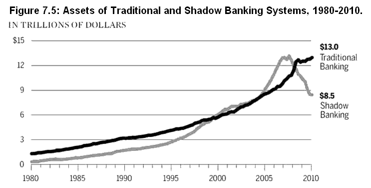
Chapter 8: Securitization, Derivatives, and Leverage
George H. Blackford © 2009, last updated 5/1/2014
Securitization is a process by which illiquid assets—that is, assets that cannot be easily sold and, hence, converted into cash in a timely manner without a significant reduction in price—are converted into liquid assets that can be quickly sold and converted into cash without a significant reduction in price. We touched on the basics of securitization in Chapter 7 in our discussion of the way finance companies were able to gain access to the money market by setting up a Special Purpose Vehicle (SPV) to secure financing in the Asset-backed Commercial Paper (ABCP) market. In so doing they were able to convert their illiquid assets (the loans made to their customers) into liquid assets (the ABCP issued by the SPV) that were easily sold in the money market.
As was indicated in Chapter 7, the basic mechanism by which securitization is accomplished is fairly simple:
The originator of the securitization process creates a Special Purpose Vehicle (SPV) by forming a corporation (generally "off shore" in some country such as in the Cayman Islands to avoid regulation and taxes) for the purpose of purchasing the assets to be securitized. The originator of this process is referred to as the sponsor of the SPV.
The sponsor sells the assets to be securitized to the SPV.
The SPV places these assets in a trust pledging the revenue from the assets as collateral for the securities issued by the SPV. These securities are referred to as Asset-backed Securities (ABSs) and are either collateralized bonds or collateralized money market paper depending on whether their term to maturity is more than or less than a year.
The proceeds from the sale of the securities issued by the SPV are used to pay the sponsor for the assets it sold to the SPV.
Virtually all illiquid assets that generate an income stream have been securitized in this way since the 1980s including such things as automobile loans, credit card debt, accounts receivables, student loans, and residential and commercial mortgages, but of particular interest to us here is the securitization of mortgages.
Mortgage Backed Securities
Before 1938, home mortgages were highly illiquid assets, the reason being it is very difficult for a third party to judge the quality of a mortgage. When a bank originates a mortgage it has a very good idea of the creditworthiness of the borrower, the quality of the real estate that is the collateral for the mortgage, and the characteristics of the neighborhood in which the real estate is located. The further one gets from the bank that originated the mortgage the less one knows about these things. As a result, the secondary market for mortgages—that is, the market in which existing mortgages are bought and sold—tended to be very local which made it difficult for people in smaller communities to obtain mortgages for the purpose of purchasing homes.
In 1938 the Federal National Mortgage Association (Fannie Mae) was created as a government agency to facilitate home ownership by providing a secondary market for government insured mortgages. In 1968 Fannie Mae was privatized as a Government Sponsored Enterprise (GSE), and in 1970 the Federal Home Loan Mortgage Corporation (Freddie Mac) was chartered as a GSE to provide a secondary market for non-government insured mortgages, and Fannie Mae was given this mission as well. In the meantime the Government National Mortgage Association (Ginnie Mae) was created as a government agency to replace Fannie Mae in the market for federally insured mortgages. Ginnie Mae is a government owned corporation within the Department of Housing and Urban Development (HUD), whereas, Fannie Mae and Freddie Mac are private corporations that were created by the government and then sold to the private sector.
The GSEs and Ginnie Mae worked closely with mortgage originators, mostly banks and thrifts (i.e., savings banks and savings and loan associations), to maintain and improve underwriting standards (i.e., the standards by which loans are made) and were very successful in providing a nationwide mortgage market by purchasing mortgages from originators that met their underwriting requirements. This, in turn, greatly facilitated home ownership throughout the country.
Originally the GSEs financed their operations by selling uncollateralized bonds in the capital market to obtain the funds necessary to purchase mortgages from their originators, but in the 1970s they began securitizing the mortgages they purchased by sponsoring Special Purpose Vehicle and having their SPVs issue bonds collateralized by the revenues generated from the mortgages they had purchased. The GSEs guaranteed the mortgages they sold to the SPVs they sponsored, and the bonds issued by their SPVs are referred to as agency Mortgage-Backed Securities or agency MBSs.
The GSEs dominated the secondary mortgage market through the 1990s, but in the 1980s private companies began securitizing mortgages as well. The bonds issued by the SPVs sponsored by private companies are referred to as private-label Mortgage-Backed Securities or private-label MBSs. Private securitizers—mostly investment banks, depository institutions, and mortgage banks—did not guarantee the mortgages they sold to their SPVs, and, as a result, private securitizers had to offer credit enhancements to minimize the interest rates they would have to pay on the MBSs they issued.
One method of credit enhancement was to over collateralize the MBSs they issued so that the face value of the MBSs the SPV issued was below the face value of the mortgages held as collateral for their MBSs. A second method was to provide an excess spread on the rate of interest received from the mortgages over the rate of interest paid on the MBSs so the amount of money taken in from the mortgages that collateralized their MBSs exceeded the amount the SPV was obligated to pay to bondholders. However, the most important of these enhancements was subordination whereby the MBSs issued by the privately sponsored SPVs were structured in a hierarchy of tranches (a French word meaning slices) such that those MBSs in a lower tranche were subordinate to those in a higher tranche.
The way subordination works is that the MBSs issued by the SPV are broken down into senior tranches which have first claim to the income received from the mortgages held by the SPV, junior tranches (also called mezzanine tranches) which have a claim to this income only after the MBSs in the senior tranches have been paid, and equity tranches (also called residual tranches) which are paid only after the MBSs in the senior and junior tranches have been paid. This structure gives the MBSs in the senior and junior tranches protection against default on the mortgages held by the SPV in that the equity tranche has to be completely wiped out by mortgage defaults on the underlying mortgages before the income and principal payments available to service senior and junior tranches will be affected, and it gives even more protection to the MBSs in the senior trance as both the equity and junior tranches have to be wiped out before the income available to service the senior tranche will be affected.
The way in which MBSs are structured is illustrated in Figure 8.1 which shows the structure of the CMLTI 206-NC2 offering sponsored by Citigroup in 2006.
Figure 8.1: Structure of the CMLTI 2006-NC2 MBS Offering.
Tranches
Amount*
Rating
% of Total
Cumulative %
Senior
Investment
Grade
$737.0
AAA
78.0%
78.0%
Junior
Investment
Grade
$97.5
AA
10.3%
88.3%
$43.6
A
4.6%
92.9%
$30.2
BBB
3.1%
96.0%
Junior Non- Investment
Grade
$24.6
BB
2.6%
98.6%
Equity
$13.3
Not Rated
1.4%
100%
Total
$946.2
100%
Source: Financial Crisis Inquire Report, Security Exchange Commission.
*millions of dollars
This offering was backed by 4,499 mortgages with a principal value or $947 million, and was described as a “typical deal” in the final report of the Financial Crisis Inquire Commission. As is shown in this figure, 78% of the MBSs in this offering were investment grade securities in the Senior Investment Grade tranche that were rated AAA by the rating agency Standard & Poor’s. Another 18% were in the Junior Investment Grade tranches that were rated BBB or above, but less than AAA, which brought the total of the investment grade securities in this offering to 96%. The 2.4% of the offering in the Junior Non-Investment Grade tranches that received a BB rating or below held a junk bond status, and the Equity tranches made up 1.4% of the offering.[8.1]
By structuring their offerings in this way, the sponsors of private-label Mortgage-Backed Securities were able to compete with the GSEs even though the sponsors of the private-label MBSs did not guarantee the mortgages that backed their MBSs. As a result, private-label MBSs began to increase their share of the Mortgage-Backed Securities market dramatically in the 2000s, but there was a catch: Virtually all of the demand was for the highest rated securities in the offerings, and there was relatively little demand for those that were lower rated. (FCIC Smith) This led to a problem.
For securitization to work, all of the tranches in an offering must be sold. Otherwise, there’s not enough money to purchase the collateral needed to make the offering viable. When the lower rated securities can’t be sold elsewhere, the sponsor of the offering is forced to purchase them. This limits the ability of the sponsoring institution to sponsor new offerings since its purchases from its previous offerings must be financed. The ability to finance these purchases is limited by capital requirements in the case of a regulated institution such as an investment bank, or by margin requirements in the case of an unregulated institution such as a hedge fund. When the sponsoring institutions reach their funding limits, they can no longer sponsor new MBS offerings. To solve this problem the sponsors of Mortgage-Backed Securities turned to alchemy.
Collateralized Debt Obligations
Collateralized Debt Obligations (CDOs) are created in the same way Mortgage-Backed Securities are created and are divided into subordinate tranches with the equity and junior tranches being paid only after the senior tranches are paid, and the equity tranches being paid only after the senior and junior tranches are paid just as MBSs are structured. In addition, CDO offerings were rated similarly by the rating agencies with 95% or so of the offering rated investment grade (BBB or higher) and as much as 80% of the offering in the senior, investment-grade tranches receiving a triple-A rating.
The fundamental difference between Collateralized Debt Obligations and Mortgage-Backed Securities is in the nature of the collateral. While MBSs are backed only by mortgages, CDOs use a variety of debt obligations for collateral—bonds, loans, and other Asset-backed Securities (ABSs)—rather than a single kind of financial instrument. (FCIC)
Until the 2000s, CDOs were a relatively obscure financial product confined to a relatively small market, but in the early 2000s the CDO market simply exploded. From 2003 to 2006 it increased more than seven fold as it went from $30 billion to $225 billion in just three years. In the process, CDOs transformed the mortgage market by increasing the demand for MBSs in the lower rated tranches. In 2004, CDOs were the dominate buyer of BBB-rated MBSs, and in 2005 they purchased virtually all of the BBB tranches of these securities. Between 2003 and 2007 over $4 trillion Mortgage-Backed Securities were created and some $700 billion of CDOs that contained lower rated tranches of MBSs as collateral were created as well. (FCIC)
The alchemy involved in this process should be apparent. By taking the lower rated MBSs and using them as collateral for CDOs, the sponsors of the SPVs that offered these CDOs for sale were able to convert as much as 80% of the BBB or BB rated MBSs held as collateral in their SPVs into triple-A rated securities in the form of AAA rated CDOs. They were, indeed, able to make a silk purse out of a sow’s ear—or so it seemed—and the alchemy didn’t end there. CDOs were often structured with the lower rated tranches of other CDOs as part of their collateral. CDOs with 80% or more of their collateral in the form of lower rated tranches of other CDOs were referred to as CDOs squared, and by this sleight of hand the sponsors of the SPVs were able to convert more than 60% of the lower rated CDO tranches held in their portfolio of collateral into triple-A rated CDOs. (FCIC)
Collateralized Debt Obligations fueled the mortgage market as it expanded in the mid 2000s in that CDOs allowed the sponsors of MBSs to keep the lower rated tranches of the MBSs that they couldn’t sell otherwise off their books. This freed up capital and, thus, allowed them to expand the creation of MBSs beyond what they would have been able to if the CDO market had not existed.
Derivatives and Leverage
Leverage is a term used to describe methods by which investors can enhance their return on equity capital. The most common kind of leverage is the kind discussed above and in Chapter 5 and Chapter 6 and again in Chapter 9, namely, borrowing money to increase the amount to invest. This kind of leverage is referred to as balance sheet or debt leverage where the amount of leverage is measured by the debt to equity ratio—that is, by the value of the amount borrowed by the investor divided by the value of the equity owned by the investor. There is another kind of leverage that can be used to increase the return on equity capital, namely, that which is obtained through the use of derivatives. Derivatives are contracts that derive their value from some underlying asset or collection of assets. They are used either to provide a hedge against a potential loss or to speculate on future events.
Option Contracts
Perhaps, the simplest derivative to understand is an option contract. An option contract is a financial instrument that gives the holder of the contract the right, but not an obligation, to either buy or sell, depending on the kind of option, an asset at a specified price during a specified period of time. An option to purchase an asset is a call option. An option to sell an asset is a put option. While an option does not obligate the holder of the option in any way, if the holder of the option chooses to exercise the option during the specified time period the writer of the option is obligated to sell, in the case of a call option, or to purchase, in the case of a put option, the asset being optioned at the specified price.
For example, if you purchase a 30-day option to purchase 100 shares of IBM stock at $100/share—a 30-day call option for 100 shares of IBM stock at $100/share—this gives you the right to purchase 100 shares of IBM stock for $100/share at any time during the next 30 days. At the same time, it obligates the writer of the option to sell 100 shares of IBM stock to you at $100/share at any time you choose during the next 30 days.
If you purchase a 30-day option to sell 100 shares of IBM stock for $100/share at any time during the next 30 days—a 30-day put option for 100 shares of IBM stock at $100/share—this gives you the right to sell 100 shares of IBM stock at $100/share at any time during the next 30 days. At the same time it obligates the writer of the option to purchase 100 shares of IBM stock from you at $100/share at any time you choose during the next 30 days.
If you own 100 shares of IBM stock that is worth $100/share you can use an option to hedge the risk of the value of your stock falling over the next six months by purchasing a 6-month put option that gives you the right to sell 100 shares of IBM stock at $100/share at any time during the next six months. Having purchased such an option, if the price of IBM stock should fall to, say, $50/share you would be protected from that loss. Your $5,000 loss in the value of your stock would be exactly offset by the $5,000 gain in the value of your option that gives you the right to sell your 100 shares of IBM stock at $100/share. Your only loss would be the price you had to pay for the option.
You can also use options to speculate on the price of IBM stock even if you don’t own the stock. Suppose you believe that IBM stock is going to double in value over the next six months. You can take advantage of this expectation either by purchasing IBM stock directly or by purchasing a 6-month call option for IBM stock. If the price of IBM stock is $100/share it will cost you $10,000 to purchase 100 shares of stock. If you purchase the stock and are right about the price of IBM doubling over the next six months, the price of your stock will increase to $200/share, your 100 shares of IBM stock will be worth $20,000, and you will make a $10,000 profit.
Alternatively, if the price of a 6-month call option to purchase IBM stock for $100/share is $10/share, that same $10,000 you have to invest could be used to purchase an option that would give you the right to purchase 1,000 shares of IBM stock for $100/share. If the price of IBM stock were to double the value of your option would increase from the $10,000 that you paid for it to $100,000 since your option gives you the right to purchase $200,000 worth of IBM stock for just $100,000. As a result, you would be able to make a $90,000 profit ($200,000 - $100,000 -$10,000) by investing your $10,000 in the option as opposed to a $10,000 profit by investing in the stock. Thus, purchasing the option allows you to leverage your $10,000 investment by increasing your profits 9 times what you would be able to make by buying the stock directly.
Just as debt leverage increases your risk of loss as it increases your potential profit, the same is true for derivative leverage. Even though your potential loss is limited to $10,000 whichever investment your chose to make in the above example, if you chose to invest in an option you will lose the entire $10,000 if the price of IBM fails to increase above $100. You will not lose your entire $10,000 investment if you chose to purchase IBM stock directly unless the price of IBM stock goes to zero.
Futures Contracts
Historically, derivatives in the form of futures contracts—an agreement to buy or sell something at a specific date and price in the future—have been around for over a hundred and fifty years, and just as with options contracts, futures contracts can be used to hedge against a potential loss or to speculate on changes in prices.
To see how a futures contract can be used to hedge against a potential loss, consider the plight of a farmer who knows approximately what it will cost to plant a particular crop in the spring and how much product he will have available to sell when it is harvested, but has no way of knowing what the price of that crop will be when he brings it to market. If he plants the wrong crop he will lose money if the price at harvest time is below his costs of production. One way he can hedge against this possibility is by entering into a contract in the spring with a miller to sell his crop in the fall at an agreed upon price. By entering into this kind of contract both the farmer and the miller are able to protect themselves against adverse changes in prices when crops are brought to market in the fall.
As was noted, futures contracts can also be used to speculate on changes in prices. If the price of wheat is $2/bushel in May and you think it will be $4/bushel in the September you can take advantage of this situation by buying wheat today, storing it until September and selling it in September at whatever the price turns out to be. If your expectation is correct and the price in September is $4/bushel you will be able to make a profit of $2/bushel on each bushel of wheat you purchase and store, less the cost of storing the wheat from June to September. If it costs you $1/bushel to store the wheat your net profit will be $1/bushel.
Now suppose that you can enter into a futures contract to purchase wheat at $3/bushel in September, a price that is equal to the price of wheat today plus the cost of storing wheat that exists today until September. If you enter into this contract and your expectation is correct and the price in September is $4/bushel you will make the same profit of $1/bushel when you purchase the wheat in September at $3/bushel and resell it at $4/bushel, less, of course, the cost of the commission to the broker who arranged the contract. There are, however, a number of important differences.
To begin with, when you purchase a futures contract you don't have to actually buy any wheat in order to make a profit. As the price of wheat approaches $4/bushel in September, the value of your contract will approach $1/bushel since that’s the profit you can make on it when it comes due. As a result, when your contract comes due in September you will be able to sell your contract to someone who actually wants to buy wheat or to someone who has contracted to sell wheat and wants to close out his or her contract to sell by buying an offsetting contract to buy without having to actually come up with the wheat needed to fulfill his or her contract to sell. This makes speculating through futures contracts much less time consuming and less of a bother than actually purchasing and storing the commodity involved.
Second, it you wish to purchase, say, 10,000 bushels of wheat to speculate on the price of wheat in this situation you will have to come up with $20,000 to purchase the wheat and an additional $10,000 to store the wheat until September for a total of $30,000. If the price of wheat is $2/bushel in May and you can purchase a futures contract to purchase 10,000 bushels of wheat at $3/bushel or less in September (the price in May plus the cost of storing the wheat until September) there is no reason for you to actually purchase the wheat since you will make at at least as much profit or more if you purchase the futures contract that commits you to purchase the wheat in September for $3/bushel as you will if you purchase the wheat at $2/bushel in May and store it until September.
In addition, you will have to come up with much less cash to purchase the futures contract than you will have to come up with to purchase the wheat. When you purchase a futures contract you only have to come up with the commission paid to the broker and enough collateral to convince the counterparty to your contract that you will, in fact, live up to your end of the contract. The collateral posted on a futures contract is referred to as the margin, and it can be as little as 10% or even as low as 5% of the value of the wheat covered by the contract. That means that instead of having to come up with $30,000 to purchase and store 10,000 bushels of wheat you can place the same bet on the price of wheat in September by coming up with only $3,000 (ignoring the broker's commission which I will do from now on to simplify the exposition) if the margin is 10% or only $1,500 if the margin is 5%.
The potential leverage here should be obvious. If you have $30,000 to invest in this speculative endeavor you have the option of using that $30,000 to purchase 10,000 bushels of wheat and storing it, or at a 10% margin you can use your $30,000 as collateral for 10 futures contracts that commit you to purchase 10,000 bushels of wheat each. If you are right and the price of wheat is $4/bushel in September you will make a $10,000 profit on the 10,000 bushels of wheat you purchased with your $30,000 if you chose the first option, and you will make a $100,000 profit on the 100,000 bushels of wheat you have committed yourself to purchase with your $30,000 if you chose the second option. In other words, you can leverage your investment tenfold by purchasing the futures contracts at a 10% margin. If the margin is 5% you can leverage your investment twentyfold by purchasing 20 contracts that commit you to purchase 200,000 bushels of wheat.
Finally, it should be obvious that the ability to purchase futures contracts not only leverages you profits, it leverages your risk as well. If you purchase the wheat in the above example, and the price falls to $1/bushel instead or increasing to $4/bushel as you had expected, you will lose the $10,000 you spent on storage and an additional $10,000 when you are stuck with 10,000 bushels of wheat you bought at $2/bushel that can now only be sold at $1/bushel. This 67% loss on your investment may sound grim, but if you had instead purchased 10 futures contracts on a 10% margin that committed you to purchase 100,000 bushels of wheat at $3/bushel and you can only sell that wheat for $1/bushel on its due date you are out $200,000. That's a 667% loss on your investment. If you had purchased 20 contracts on a 5% margin your loss would be $400,000 on your $30,000 investment. That's more than 13 times the amount you had planned to invest in the first place!
This brings us to a very important point: When derivatives are used to hedge against a risk of potential loss the risk that is hedged is transferred from one party of the derivative contract to the other. There is no increase in risk in the system as a whole, and there even may be a reduction in risk in the system as a whole if the risk is transferred from an individual or institution that is less able to cope with the potential loss to an individual or institution that is better able to cope with the potential loss. As a result, using derivatives to hedge against a potential loss can have the effect of increasing the stability of the economic system as a whole. This is not the case when derivatives are used for pure speculation.
When derivatives are used for pure speculation where neither party is hedging against a risk of potential loss, both parties to the contract assume risk that they otherwise would not have assumed. There is no transfer of risk, and the total risk of potential loss in the system increases. This should be clear from the example above. When you purchase an option on 100 shares of IBM stock you do not own from a writer who is not hedging against a potential loss there is no transfer of risk. Both you and the option writer are taking on risks of loss that you would not otherwise have. The same is true in the futures market when neither party is hedging against a potential loss.
The fact that speculators add to the liquidity of the market and thereby enhance the ability of other participants to hedge does not negate the fact that pure speculation increases the risk in the system as a whole and, as a result, reduces the stability of the system as a whole.
While in theory, pure speculation is a zero-sum game where the losses of one party are equal to the gains by another and all that occurs as a result of speculation is a transfer of wealth from one group of individuals to another, in practice this is not necessarily the case and often is, in fact, not the case. This theory ignores the possibility of default on the part of those who speculate and the damage that can be done to those who are directly and indirectly affected by the speculative bubbles that are created as a result of speculation.
When speculative bubbles burst, the inability of those affected to meet their contractual obligations can have a cascading effect that brings the entire economic system to its knees. The history of this being so goes back at least 800 years. (Kindleberger MacKay Graeber) The recognition of this problem led to the establishment of exchanges and clearinghouses. These are institutions that were designed to minimize the risk of default and also to minimize the risk of manipulation and fraud within the market.
Exchanges and Clearinghouses
The markets for options, futures, and many other derivatives have become highly efficient as these contracts have been standardized and are widely traded on exchanges where an exchange is simply a central meeting place where trading takes place. The importance of an exchange is that it provides a place where trading is in the open, and all of the participants in the market can see the quantities bought and sold and the prices at which trades are made. This kind of openness, or what is referred to as transparency in the market, is designed to minimize fraud and the ability of traders to manipulate prices.
In addition, the risk of default on derivative contracts has been minimized through the establishment of clearinghouses whereby the contracts agreed upon between individuals at the exchange are cleared through a separate corporation, and that corporation—the clearing house—becomes the counterparty to the buyers and sellers in the contracts that are agreed upon in the exchange. The way an exchange and clearinghouse work to minimize the creation of speculative bubbles and risk of default for those derivatives that are traded through an exchange with a clearinghouse can be seen by examining the way a futures contract comes into being.
If you wish to enter into a contract to buy (or sell) wheat or some other commodity at some point in the future you go to your broker and place an order. Your broker submits your order to the exchange where all of the offers to buy and sell are submitted by the brokers that are members of that exchange. The brokers’ traders on the floor of the exchange match the offers to buy with the offers to sell where the prices at which the commodities are to be bought and sold in the future are determined through an auction process among the traders.
At the end of each trading day the contracts that have been agreed upon are submitted to the clearinghouse to be cleared, and the cash transactions between the brokers and the clearinghouse are settled. The outstanding contracts held by each broker's clients are then revalued in accordance with the prices set during the day, and each broker is required pay any balance its clients may have accumulated in order to maintain the margin required on their contracts to the clearinghouse as a result of the day’s trading. Once the trades of the day have been reconciled, and the margin requirements have been met by the members of the exchange, the contracts between the clients of the brokers are dissolved, and the clearing house becomes the counterparty to each of the contracts the clients have entered into. Your broker then delivers to you your contract with the clearinghouse that you sought to enter into.
The efficiency of this system arises from the fact that all of the participants in the market are policed by the brokers, by the exchange, by the clearing house, and the entire process is regulated by the government. All transactions are executed publicly on the floor of the exchange, available for all to see, and changes in the values of the outstanding contracts are reconciled each day in order to maintain the collateral each broker must deposit with the clearinghouse as determined by the margin requirement on the contracts its clients have with the clearinghouse.
You are legally responsible to your broker to perform on your contract and your broker is legally responsible for your performance to the clearinghouse as well. That means that if you default on your contract your broker is responsible to make that contract good to the clearinghouse, and if your broker defaults to the clearinghouse, the clearinghouse is on the hook to make that contract good to whomever made it with you. That protects the original counterparty to your contract from default on your part, and it also protects you from default on the part of the original counterparty to your contract since the counterparty’s broker is responsible for the contract his client made with you as is the clearinghouse.
The only situation in which your contract will not be honored is if the clearinghouse were to default. This is clearly a possibility, but the fact that a) the changes in the values of all outstanding contracts between brokers and the clearinghouse must be reconciled each day, b) each broker is required to maintain the margin on its clients contracts with the clearinghouse as the values of its clients contracts fluctuate each day, c) clients are required to maintain the margin on their contracts with their brokers as the value of the contracts fluctuate each day, and c) the fact that the behavior of all of the participants in the market is strictly regulated by the government minimizes this possibility.
Trading in derivative contracts has been regulated by the government, in one way or another, since the 1880s, and trading in commodities options was banned altogether in 1936. The government sets the margin requirement that must be maintained against your account with your broker as well as against your broker’s account with the clearinghouse, as it does for all the clients and brokers in the system, in order to assure that each client will be able to make good to his or her broker and each broker will be able to make good to the clearinghouse on a daily basis any losses that may be realized. In addition, fraudulent, misleading, manipulative, and reckless or unsafe practices that threaten the solvency of the clearinghouse are prohibited and enforced through government regulations and regulators.
Credit Default Swaps and Synthetic CDOs
Even though derivatives have been around for a very long time, the way in which they have been used has changed dramatically over the past forty years. Prior to the 1970s, futures contracts were used for commodities and, as has been noted, options trading in commodities was outlawed. In the 1970s futures contracts for financial assets were introduced, and the ban on option trading in commodities was lifted in 1981. Option trading was subsequently extended to include financial assets and foreign exchange as well as commodities, and new kinds of options and futures contracts were created—contracts based on indices of commodity and financial asset prices as opposed to those based on individual commodities and financial assets.
At the same time, much of the trading in derivatives has moved from the exchange/clearinghouse environment to the over-the-counter market where contracts are not standardized and are made directly between individuals and institutions without the protection of a clearinghouse, with very little government regulation, and with very little if any transparency. In addition, an entirely new category of derivative came into being, the swap, whereby contracts were devised that allowed income streams generated by assets to be exchanged in domestic as well as in foreign currencies, and in 1997 the Credit Default Swap was born.
Credit Default Swaps
A Credit Default Swap (CDS) is a kind of insurance contract wherein the seller of a CDS agrees to compensate the buyer against the consequence of an adverse credit event such as the issuer of a bond defaulting on its interest or principal payment. The buyer pays the seller a quarterly or biannual premium for the protection provided by the seller where the protection generally consists of an agreed upon, lump-sum payment from the seller to the buyer should the credit event (e.g., default) occur.
The market for Credit Default Swaps came into being in the late 1990s, and this market played a crucial role in the mortgage market in the 2000s. In particular, it played a crucial role in the markets for Mortgage Backed Securities and Collateralized Debt Obligations since CDSs made MBSs and CDOs more attractive to those who sought protection against the risk of these kinds of bonds defaulting. Regulated institutions such as banks, for example, could reduce their capital requirements by purchasing credit default protection against the MBSs and CDOs they held, and hedge funds and other financial institutions could use CDSs to hedge positions that involved MBSs, CDOs, or other forms of Asset Backed Securities.
Insurance is generally subject to government regulations that force insurance companies to maintain reserves commensurate with their obligations to policy holders. Government regulations also outlaw insurance policies being issued to people who do not have an insurable interest in what is being insured and, in particular, they bar people from obtaining insurance on property they do not own. In addition, people are generally not allowed to insure property for more than the damages they will incurred if the property is lost or damaged. But even though CDSs are a kind of insurance, the Commodity Futures Modernization Act (CFMA) passed in 2000 explicitly blocked regulation of the market for Credit Default Swaps. This made it possible for financial institutions to purchase and sell Credit Default Swaps to insure debt instruments that were not owned by the purchaser, to purchase and sell multiple CDS contracts against these same instruments, and for financial institutions to sell CDS insurance contracts without setting aside reserves. It also made synthetic CDOs possible.
Synthetic CDOs
A Synthetic CDO is created and structured in the same way a MBS or an ordinary CDO is created and structured, but there are a number of important differences. The first is that the Special Purpose Vehicles that create synthetic CDOs sell Credit Default Swaps and hold safe securities (such as government bonds) as collateral instead of actual mortgages or MBSs. The way this works is the sponsor of a synthetic CDO incorporates a SPV and puts together a list of MBSs for which the sponsor wishes to sell default protection. The SPV then sells Credit Default Swaps to those who are willing to pay a premium for default protection on the listed securities.
The SPV then structures an offering of synthetic CDO tranches similar to the structure of the MBS offering shown in Figure 8.1 with the same kind of subordinated payout to the investors in the synthetic CDO securities that is used in the payout structure of ordinary CDOs and MBSs. The proceeds from the sale of the synthetic CDOs are, in turn, invested in safe securities. These safe securities become the collateral held by the SPV. The interest payments received from these securities combined with the premium payments received from the CDS contracts sold by the SPV provide the funds needed to make the interest and principal payments on the synthetic CDOs purchased by investors.
This brings us to the second way in which synthetic CDOs differ from ordinary CDOs. There are two kinds of investors in a synthetic CDO. The first is the fully-funded investor described above. Fully-funded investors are required to put up 100% of the money they are putting at risk. They actually lend money to the SPV in order to receive interest payments on the CDOs they purchase. This money is used to purchase the safe assets that the SPV uses as collateral. The second kind of investor is the unfunded investor.
Unfunded investors are not required to put money up front and do not lend money to the SPV. Instead, unfunded investors, in effect, sell credit-default protection to the SPV—protection that insures payment to those who purchased Credit Default Swaps from the SPV. All other investors are subordinate to the unfunded investors in a synthetic CDO offering, which means, of course, that all other investors in a synthetic CDO get paid after the unfunded investors get paid. This adds another level of subordination to the tranche structure of the synthetic CDOs, namely, what is referred to as the Super-Senior tranche that is sold to unfunded investors.[8.2]
The way in which synthetic CDOs are structured is illustrated in Figure 8.2 which shows the structure of the ABACUS 2004-2 offering sponsored by Goldman Sachs in 2004. In spite of the obvious differences between Figure 8.2 and Figure 8.1, they are very much the same in that 87% of the synthetic CDOs in Figure 8.2 are rated AAA or are subordinated above the triple-A tranches compared to 78% of the MBSs in Figure 8.1, and only 5% are rated less than investment grade in Figure 8.2 compared to 4% in Figure 8.1.
Figure 8.2: Structure of the ABACUS 2004-2 Synthetic CDO Offering.
Tranches
Amount*
Rating
% of Total
Cumulative %
Super Senior
Unfunded
$850.0
Not Rated
85.0%
85.0%
Senior
Fully Funded
Investment
Grade
$20.0
AAA
2.0%
87.0%
Junior
Fully Funded
Investment
Grade
$40.0
AA
4.0%
91.0%
$30.0
A
3.0%
94.0%
$10.0
BBB
1.0%
95.0%
Equity
$50.0
Not Rated
5.0%
100%
Total
$1,000.0
100%
Source: Financial Crisis Inquire Commission.
*millions of dollars
In terms of the payout from the investment, there is no difference between a synthetic CDO that sells CDSs and holds safe securities for collateral and an ordinary CDO that holds the actual MBSs that underlie the CDSs sold by the synthetic CDOs. If there are no defaults in the underlying MBSs the CDO investors will all get paid whether the CDO is synthetic or not. If some of the underlying MBSs default, some of the safe securities will have to be sold to pay off the CDSs that insured those MBSs. In this situation, some of the investors who purchased the lower tranches of the synthetic CDOs will not get paid, but the same would be true if those investors had invested in the lower tranches of an ordinary CDO that actually held the MBSs that defaulted. It makes no difference from the perspective of the payout to the investor what form the CDO takes. In either case, the amount the investor gets paid or loses is the same.
There is, however, a fundamental difference between investing in a synthetic CDO and investing in an ordinary CDO in terms of the kind of investment being made. Investors who purchase ordinary CDOs are investing in the mortgage business. The money they are investing is used to purchase mortgages—albeit, indirectly by way of financing the tranches of the CDOs that are used to purchase MBSs that are used to purchase mortgages.
Investors who purchase synthetic CDOs are investing in the insurance business, not the mortgage business. The money they are investing is used to insure the debt instruments that underlie the CDSs sold by the SPV not to purchase mortgages. In addition, the collateral held by the SPV is not put up by the borrower, it is put up by the lender, and it is not held to protect those who lend by purchasing the synthetic CDOs. It is held to protect those who purchase the Credit Default Swaps that are sold by the SPV.
Not only were the fully funded investors in synthetic CDOs investing in the insurance business, they were investing in the insurance business in an unregulated market. There were no government regulations that prevent those who were buying the MBS insurance offered by the SPV from being the very same people that selected the MBSs being insured. The conflict of interest here should be obvious, especially since the people who purchased the insurance and selected the MBSs to be insured did not have to own the MBSs they had selected. They had nothing to lose if the MBSs they selected to insure went bad, and they receive a huge payout if these MBSs did in fact go bad.
Initially, the institutions that sold Credit Default Swaps were pretty much limited to AIG and a few monocline insurance companies such as MBIA and Ambac, but with the invention of the synthetic CDO the major players in the MBS and CDO markets such as J. P. Morgan and Goldman Sacks were able to secure credit protection from an ever increasing number of investors through the sale of the fully-funded, synthetic CDOs. All that was required to sell a fully-funded synthetic CDO was to find a buyer who 1) had enough money to make the purchase, 2) who sought the safety the investment-grade rating of these bonds seemed to provide, and 3) who was unable to understand exactly what it was that was being purchased. Investment-grade, fully-funded, synthetic CDOs were sold to banks, pension funds, endowment funds, hedge funds, mutual funds, insurance companies, and municipal governments throughout the country and all over the world. Virtually any entity that met the above criteria was fair game to those who sold these securities. (FCIC WSFC)
Finally, as is clear from the way in which the synthetic CDOs were structured, those who bought the unfunded, super-senior tranches were given added protection from loss by the fully-funded tranches since the fully-funded tranches were subordinated to the super-senior tranches and took the first losses. This was particularly appealing to many of the institutions that sponsored synthetic CDOs since these institutions did not have to put up cash to purchase the Super Senior tranches they had created and could receive income from these tranches without having to set aside capital to support them. As a result, many of the super-senior tranches of the synthetic CDOs ended up on the books of the financial institutions that sponsored these CDOs, much to their regret when the crisis came. In other words, these institutions assumed the risk of selling credit-default protection to the SPV, a practice that proved disastrous in the fall of 2008. (FCIC WSFC)
Shadow Banks, Derivatives, and Systemic Risk
The systemic risk the shadow banking system posed—that is, the threat to the financial and economic systems as a whole—especially when combined with an unregulated insurance market and derivatives markets that were not only unregulated but operated without exchanges or clearinghouses, should have been obvious to anyone with a reasonable understanding of the history of the financial system, but ideological blindness inspired by an almost religious faith in free markets made it impossible for policy makers and elected officials to take this risk seriously. When this blindness was combined with the fact that the vast majority of elected officials knew virtually nothing about the history of the financial system, the stage was set for a catastrophe of epic proportions.
The irony is that the first run on a shadow bank occurred ten years before the entire shadow banking system collapsed in the fall of 2008 when a run on the hedge fund Long-term Capital Management in 1998 nearly caused a worldwide financial meltdown. This run literally terrified policy makers and the entire financial community at the time, and, yet, as we will see, nothing was done to curb the excesses of the shadow banking system or to regulate the over-the-counter derivatives markets in the wake of this near catastrophe.
Endnotes
[8.1]The ratings, AAA, BBB, etc., represent the rating agencies estimate of the probability of default for the security being rated based on the historical performance of securities that have held that particular rating in the past. The ten year time horizon for the historical performance of Moody’s ratings from 1970-2010 is given in following table from Moody’s Confidence Intervals for Corporate Default Rates:
[8.2] The Super Senior tranches were only sold to the most creditworthy institutions with triple-A credit ratings such as to AIG and a few monocline insurance companies such as MBIA and Ambac—institutions that turned out, in the end, to be not so creditworthy, largely by virtue of the fact that they invested in the super senior tranches of the synthetic CDOs.
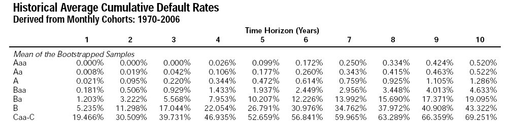
Chapter 9: LTCM and the Panic of 1998
George H. Blackford © 2009, last updated 5/1/2014
The story of Long Term Capital Management (LTCM) has been told by Roger Lowenstein in his captivating book When Genius Failed, but for those who have not had a chance to read this book I will, with a few embellishments, summarize it here.
LTCM was a hedge fund started 1994 by John Meriwether, a legendary trader who made a fortune for himself and Solomon Brothers in the 1980s. (Lewis NYT) The fund was a limited partnership where the senior partners were Meriwether along with Myron Scholes and Robert Merton, both of whom were to receive the Nobel Prize in Economics 1997; David Mullins, a former vice chairman of the Board of Governors of the Federal Reserve; Eric Rosenfeld, a former professor from Harvard's Business School; Greg Hawkins, a campaign manager for Bill Clinton in the 1980s; Victor Haghani, a former managing director at Solomon Brothers; William Kasker, a former professor from Harvard's Business School; and Larry Hilibrand along with a number of other former traders from Solomon Brothers.
This was a group of financial rock stars that claimed six Ph.D.s from MIT among their ranks and another from the University of Chicago. Wall Street was awed by their intellectual prowess and the depth of their financial expertise. They were the Dream Team of Wall Street when they began LTCM, but the saga of LTCM lasted only four years and ended as just another study in how the Best and the Brightest can lose their way.
Rise of Long Term Capital Management
The partners raised capital by investing $50 million of their own money and soliciting an additional $1.25 billion from a group of investors for a total of $1.3 billion in equity capital—at the time, the largest amount ever raised by a startup company. Their equity grew to $7 billion by the end of 1997, and, over time, they managed to borrow over $125 billion in the money market, mostly through six month repurchase agreements. (Rosenfeld) This gave LTCM an investment portfolio of over $130 billion to work with. For the first two years LTCM earned a 40 percent rate of return on their equity and in 1997 they earned 27 percent.
The success of this company was spectacular—the stuff legends are made of. At the end of 1997 LTCM paid back $2.7 billion of its capital to its investors so the partners could increase their returns. This brought its equity capital down to $4.3 billion.
Fall of Long Term Capital Management
In April 1998 LTCM's fortunes turned. By August 16, LTCM had lost $800 million, and their equity had fallen to $3.5 billion. Then on August 17, Russia devalued its currency and defaulted on its treasury's debt.
The Russian default panicked investors all over the world and led to a flight to quality, which means invertors attempted to abandon more risky assets such as speculative stocks and bonds and purchase less risky assets such as cash and Treasury securities. This led to turmoil in the world's financial markets as the prices of the assets investors wanted to sell fell. These were the very asset held by LTCM. The following Monday, LTCM lost $553 million in the markets, and their equity shrank to $2.9 billion. They continued to lose money through the end of the month as the Dow dropped 357 points on August 27 and then fell an additional 512 points as the market crashed on August 31.
By the beginning of September, LTCM'S equity had fallen to $2.28 billion—a staggering 44 percent loss during the month of August and a 52 percent loss from the beginning of the year—LTCM was rapidly approaching insolvency. What's worse, LTCM was having liquidity problems as well. Even though most of its financing was by way of relatively long-term six month repurchase agreements, it still had to roll over one sixth of this financing each month, and this was becoming more difficult. Creditors were demanding more favorable terms, and when on September 10 LTCM's clearing fund at Bear Sterns briefly dropped below its contractual minimum, Bear insisted that LTCM's partners open their books to reassure Bear that they would be able to meet their obligations in the future. If LTCM became insolvent or defaulted on a single payment all of its loans would come due. It would then be forced into bankruptcy as its creditors scrambled to seize their collateral. In addition, by September 10 LTCM's equity had fallen below $2 billion, and it was clear that to avoid insolvency it would have to raise capital either through investors or by taking in new partners. This required that LTCM open its books to potential investors or new partners as well as to Bear Sterns.
LTCM had always been a secretive company. It's partners had never opened its books to anyone, not even to its investors or largest creditors. Now the partners had no choice. They would be out of business instantly if Bear refused to clear their trades, and they estimated they would have to raise least $2 billion in capital to survive. There was no way they could raise that kind of money without opening their books to someone. After attempting to raise the funds from a number of individuals such as Warren Buffet, George Soros, Michael Dell, and a Saudi prince LTCM contacted Goldman Sacks to assist with their fundraising and—in the strictest of confidence, of course—on Monday, September 14 opened its books to Goldman Sacks.
As LTCM opened its books and news of the tenuous nature of its solvency spread around Wall Street, LTCM's situation worsened. On Monday, September 14, the day LTCM opened its books to Goldman Sacks, LTCM lost $55 million. On Tuesday, $87 million more, and then on Wednesday, September 16 it lost an additional $122 million for a total of $264 million. That was fifteen percent of their capital lost in just three days!
The problem was that LTCM was a behemoth—four times the size of the next largest hedge fund. (GAO) It was obvious to everyone that if LTCM were driven into bankruptcy its assets would have to be liquidated. Since LTCM was so large, liquidating its assets would cause the prices of its assets to fall. Anyone that owned the same assets as LTCM would lose money if they still owned them in the event LTCM went under. This provided a powerful incentive for other institutions to sell their holdings of these assets before LTCM was forced to sell its holdings. Even worse, it was also obvious it would be possible to profit from LTCM's demise by trading against it, that is, by taking positions in the market that would make money if LTCM was forced to liquidate its portfolio. Both of these activities caused the prices of LTCM's assets to fall even faster than they otherwise would have. As a result, no one wanted to invest in, or be in debt to LTCM, and just about everyone who could was trying to make money off of their demise.
By September 16, the partner's equity had fallen to $1.5 billion, and the situation was becoming desperate. The partners estimated it would now take $4 billion in additional capital to save the company—twice what they thought it would take just three days before. At that point LTCM decided it would be best to brief the Federal Reserve on their situation. A call was made and a meeting was set for following Sunday, September 20.
Bailout of Long Term Capital Management
LTCM was not the only institution losing money during this period that found itself in serious financial difficulties. Most of the other hedge funds lost money as well and many folded. Investment banks, which by then were making money from the same kinds of investment strategies as LTCM, had financial problems as well, as did commercial banks and bank holding companies, but none of these other institutions had LTCM's problems. Commercial banks had deposit insurance to protect them from a run and access to the Fed to provide them with cash. Investment banks had sources of income other than their investment portfolios that were sufficient to tide them through. LTCM was not a bank; it had no insured source of funds and could not borrow from the Fed. The only source of funds available to it was its investment portfolio and the money market. (PWG) But what made LTCM unique was the size of its portfolio.
LTCM's portfolio was well over $100 billion on September 20, 1998. In addition, as the representatives of the Federal Reserve looked at LTCM's books they discovered LTCM had huge positions in derivatives which, as is explained in the Chapter 8, are financial instruments such as an option that have no intrinsic value in themselves but, rather, derive their value from the value of underlying assets. They are contracts between two parties, each of which is a counterparty to the other, and LTCM had entered into over 60 thousand derivative contracts with some 75 different institutions. The notional value of the assets underlying these contracts was well over $1.5 trillion! (GAO) This amounted to some five percent of the entire world market. In addition, LTCM financed most of its $100 billion in assets with some 40 thousand repurchase agreements which had counterparties as well. To make things worse, LTCM's investments and derivative commitments—and the counterparties on the other side of these contracts—were in markets all over the world: in Great Britain, Denmark, Sweden, Switzerland, Germany, France, Italy, Spain, the Netherlands, Belgium, and Russia; in New Zealand, Hong Kong China, Taiwan, Thailand, Malaysia, and the Philippines; and in Brazil, Argentina, Mexico, and Venezuela.
It was clear that if LTCM were to fail it would seriously disrupt the world's financial markets. Not only did LTCM's seventeen largest creditors—banks such as Merrill Lynch, Morgan Stanley Dean Witter, Goldman Sachs, Salomon Smith Barney—stand to lose as much as $5 billion directly if LTCM were forced into bankruptcy, if LTCM was forced to liquidate its portfolio its collateralized creditors would be forced to claim and sell their collateral, and their derivative counterparties would be forced to scrambled to protect themselves from the vulnerable positions they found themselves in as a result of LTCM's default on over a trillion dollars worth of derivatives. This kind of chaos in the financial market would undoubtedly cause asset prices to spiral downward all over the world and where and when they would stop falling no one could know. It was feared that such an event would cause a worldwide recession, and that an effort should be made to keep this from happening. The question was what?
It was not at all clear that anything could be done to save LTCM. Investors and speculators all over the world were trading against LTCM making the situation worse by the day, and given its liquidity problem and the rate at which it was losing equity, it was unlikely LTCM could remain solvent for another week or liquid enough to avoid defaulting on one of its obligations and being driven into bankruptcy. It would be impossible to find outside investors willing to invest $4 billion in LTCM under these circumstances. At the same time LTCM's portfolio was so large and so complicated that any an attempt to liquidate it in an orderly way would cause a panic. The only option that seemed even feasible was to get LTCM's major creditors together to see if they could find a way to raise the $4 billion in capital necessary to save LTCM. But there was no guarantee that even this would solve the problem.
Even though LTCM's major creditors, mostly large Wall Street banks, had the most to lose, at least directly, if LTCM went bankrupt, it was not at all likely they would be willing to put up the $4 billion in capital necessary to keep LTCM afloat. After all, that would be throwing good money after bad, and that's not how Wall Street bankers got to be Wall Street bankers. Their basic instinct would be to force LTCM into bankruptcy and feed on its carcass. Nevertheless, by Tuesday the situation seemed desperate enough to make this straw worth grasping. LTCM had lost $553 million on Monday, September 21—an amount equal to its entire loss for the month of August—and by the end of the trading day on Tuesday it had lost $152 million more. Its equity capital now stood at $773 million. Given the circumstances, it was felt that at least an effort should be made to see if LTCM's creditors would bail it out, and an emergency meeting of LTCM's 16 largest creditors was scheduled for 8:00 that evening to take place at the Federal Reserve Bank in New York City.
At the meeting a plan was presented by which a consortium of the 16 banks present would attempt to save LTCM by investing $250 million each in order to raise the $4 billion needed to end the run on LTCM. Everyone agreed that the situation was serious, but there was little agreement on anything else. Some wanted to just let LTCM go down and take their chances, but no one could be certain the collapse of LTCM wouldn't take them down with it, and most were terrified by the prospect.
Most of the bankers wanted to savage the LTCM's partners by taking over the company and leaving them with nothing, but there was no way the bankers could do this without forcing LTCM into bankruptcy. In the absence of a default on the part of LTCM, each partner would have to agree to the terms of a takeover. The partners had nothing to lose if they refused a takeover that left them with nothing so there was no reason for them to agree to it, and a default was what the bankers were trying to avoid.
Most of the bankers also wanted to fire the partners as well, but this also was problematic. LTCM's portfolio was so large and so complicated it would be very difficult for an outsider to understand it let alone manage it. No one understood this portfolio better than the partners, and in the event of a takeover the partners would have to manage it. By 11:00 only four banks were willing to commit to joining the consortium, and the meeting was adjourned until 10:00 the following morning.
On Wednesday morning the gathering was increased to include the president of the New York Stock Exchange and the executives of five British, Swiss, and French banks. In addition, the representatives of a German bank attended by way of a speakerphone. The meeting was at times acrimonious, and at a number of points the negotiations nearly collapsed, but by the end of the trading day LTCM had lost another $218 million and its equity capital had fallen to $555 million.
Gradually the bankers began to realize that this was the last chance they would have to deal with this problem, and an agreement on the terms of a takeover began to emerge. In the end it was agreed that a consortium of 14 banks would invest $3.65 billion in LTCM in exchange for 90 percent of the firm's equity. The partners would retain 10 percent of the equity and would run the firm under the supervision of the consortium. At 5:15 a phone call was placed to the partners to see if they would agree to these terms with the details to be worked out before the deal was to close on Monday, September 28. The partners agreed, and shortly after 7:00 the agreement was announced to the press.
While an agreement had been reached in principle, there was no agreement where the devil lies—the details had yet to be worked out. On Friday, 70 lawyers representing the 14 members of the consortium converged on Merrill Lynch to write the terms of the contract on a deal that had to be closed in three days—the kind of deal that usually took months. In spite of the pandemonium, after a marathon session they came up with a draft. In the meantime, LTCM lost another $155 million on Friday, and its equity capital fell to $400 million.
When the partners read the contract early Saturday morning, they were furious. As far as they were concerned there was nothing in it for them. Later that morning the partners met at a prestigious Midtown law firm to negotiate with the consortium to finalize the contract, and another marathon session began—this time 140 lawyers showed up to argue on behave of their clients. Throughout Saturday and Sunday the negotiations continued. Ironically, even if a contract acceptable to all parties were obtained, there was no guarantee it would be put into effect.
One of the conditions insisted on by the consortium was that all of LTCM's creditors sign a waiver relinquishing their right to immediate repayment of their loans to LTCM. Republic Bank, Nomura Securities, Credit Lyonnais, and Italy's foreign exchange office refused to sign. It wasn't until 5:30 on Monday afternoon that the problem of the holdouts was solved, all of the waivers that were coming in were in, and all of the disputes among the principles were resolved so that the deal to take over LTCM for $3.65 billion by the consortium of 14 banks could be closed.
The 14 banks that took control of LTCM were: Chase Manhattan Corporation; Goldman Sachs; Merrill Lynch; J.P. Morgan; Morgan Stanley Dean Witter; Salomon Smith Barney; Credit Suisse First Boston Company; Barclays; Deutsche Bank; UBS; Bankers Trust Corporation; Société Generale; Paribas; and Lehman Brothers. (GAO)
In the meantime, LTCM had another bad day. By the time the deal was closed its capital had fallen to $340 million. It lost an additional $750 million through the first half of October, then the markets rebounded, and by the end of October LTCM had stabilized. Within a year the fund was able to pay back the consortium, and by the end of 2000 LTCM had been systematically liquidated without any of the dire financial and economic consequences that were feared if LTCM had been forced into bankruptcy.
What Went Wrong
How could the financial geniuses of LTCM bring the financial world to the brink of collapse? The answer is as old as finance itself. As with poorly managed banks throughout the history of finance, LTCM's partners underestimated the risk of economic instability and over extended themselves by borrowing more than their equity capital could support in a crisis. When times were prosperous they managed to leverage their equity as much as 30 to 1. In so doing they took a risk that a financial crisis could wipe them out, but they thought that was extremely unlikely and, at the same time, for the first three years they made a fabulous amount of money.
When the crisis came and asset prices began to fall—just as in the banking world of the nineteenth century—there was no way they could sell their assets and maintain their solvency, and no one was willing to lend to them. They were caught in a modern day bank run in a nineteenth century financial environment, and there was nothing they could do to save themselves. Even the fact that they had borrowed for a relatively long time period, using six month repurchase agreements, was not enough to save them. As a result, the Fed was forced to orchestrate a takeover by a consortium of banks to head off a financial meltdown that threatened a worldwide economic crisis in its wake. That's all there was too it. As I said, it's a story as old as finance itself.
Lessons Learned From the LTCM Crisis
It is worth emphasizing that the geniuses at LTCM did not create a financial crisis that nearly caused a meltdown of the entire world's financial system because they were dumb. They knew the limitations of their models and that some unpredictable event could cause an economic catastrophe that could drive them into bankruptcy. They didn't think it would happen, but they knew it could happen. They leveraged their equity in a way that ultimately led to their downfall in spite of the risk they knew they were taking for a very simple reason: There is no other way they could have made the enormous amount of money they were able to make in the first three years of their existence without leveraging their equity in this way.
In other words, they took a chance that fortuitously threatened the financial system of the entire world because they thought it was worth it for them to take that risk. What it would mean for the rest of the world if they failed disastrously never entered their minds, at least not until the very end when it was too late to do anything about it except look for a way out of the mess they had created. What's more, there is no reason for them to have thought about what would happen to the rest of the world if they failed disastrously. No one ever got rich thinking about that sort of thing. That sort of thing is left to philosophers and is beyond the purview of free-market capitalist.
It is also important to emphasize a second reason why they leveraged their capital in that way: They leveraged their capital 30 to 1 because they could. There was no one there to stop them from doing what they thought was best for them—not the government and not their creditors—irrespective of the danger their actions posed for the rest of the world. The financial markets they operated in were unregulated. There was no law or regulation to prevent them from doing what they did, and the regulators at the time had a Panglossian faith in the efficacy of free markets to create the best of all possible economic worlds. As for their creditors, they just wanted a piece of the action. They made fortunes of their own doing business with LTCM during the prosperous years, and they too thought it was worth it for them to take the risks they were taking when they lent to LTCM at ridiculously low margins.
With no one there to stop them why shouldn't LTCM have taken that risk? Think about it for a moment. For the first three years of LTCM's existence they made over $5 billion. That works out to over $5 million a day! On some days they would lose $20 million but on others they would make $40 million. Why shouldn't they take the risk for that kind of money? After all they couldn't have made that kind of money if they hadn't taken the risk. Think of the rush it must have given them to be the master of the financial universe as they raked in all that cash. Wouldn't you take that risk for that kind of excitement?
If you answer no, you are probably one of those ordinary people who keep their money in a savings account and invest your retirement savings in a conservatively run IRA. If you had been at LTCM you would have restrained your leverage to 5 or 10 to 1 and would have been happy earning as little as $1 million a day instead of $5 million a day. You probably don't buy lottery tickets either or get excited at the prospect of a weekend in Vegas trying out a new way of counting cards at a blackjack table. In other words, you are no John Meriwether.
John Meriwether would probably not waste his time purchasing lottery tickets, but there can be no doubt that if he had the option of starting up another LTCM and doing it all over again he would start up another LTCM and do it all over again. Not only would he do it all over again, he did. On October 22, 2009 the Financial Times reported that Meriwether had embarked on this third hedge fund (JM Advisors Management) after his second fund (JWM Partners which he began less than two years after the LTCM debacle) went bust in the 2008 financial crisis. And the world is full of John Meriwethers.
Some people are movers and shakers. They are the people who get things done and are prepared to assume the risks necessary to get things done. When they are successful in the military they are called heroes. When successful in business some are called Captains of Industry, others are called Robber Barons, and some are called both Captains of Industry and Robber Barons at the same time by different groups of people. They are also called entrepreneurs by economists, and they are not the geniuses who invent a better mousetrap that frees the world from mice. They are the geniuses who find a better way to produce that mousetrap and distribute it throughout the market so that it is available to each of us to wage our own personal war against mice. Rather than invent better mouse traps they assume the risk necessary to create a better mousetrap industry. Entrepreneurs are essential to economic growth and prosperity in a market economy. They make it happen.
Entrepreneurs include the likes of Andrew Carnegie, John D. Rockefeller, Henry Ford, Thomas Edison, J. P. Morgan, and more recently Steve Jobs, Steve Wozniak, and Bill Gates. But acknowledging the grand accomplishments of these great men doesn't mean they should be allowed to play by their own rules in free and unregulated markets. After all, among their ranks we also find the likes of Charles Ponzi, Bernie Madoff, Charles Keating, Michael Milken, Ivan Boesky, Jeff Skilling, Ken Lay, Andy Fastow, and Bernie Ebbers as well as John Meriwether, Jimmy Cayne, Richard Fuld, Franklin Raines, Daniel Mudd, Richard Syron, Martin J. Sullivan, Robert Levin, Chuck Prince, Sandy Weill, Robert Rubin, and countless others who were in charge of our financial system during the era of cowboy finance in unregulated markets that preceded the near collapse of the world's financial system in the fall of 2008.
Contrary to the propaganda of the Conservative Movement, there is no reason to believe unregulated free markets must work to the advantage of society as a whole if people are allowed to seek their own advantage in the market place or even that they will work in this way. (Smith MacKay George Marx Veblen Sinclair Roosevelt Haywood Jones Fisher Josephson Keynes Polanyi Schumpeter Boyer Galbraith Musgrave Harrington Carson Nader Domhoff Kindleberger Cody Minsky Stewart Black Zinn Stiglitz Phillips Kuttner Morris Taleb Bogle Harvey Dowd Galbraith Baker Stiglitz Klein Reinhart Fox Johnson Amy Sachs Smith Eichengreen Rodrik Skidelsky Graeber) There are innumerable ways in which markets can fail to accomplish this end, and this is particularly so when it comes to financial markets.
Sooner or later an unregulated financial market will always fail to accomplish this end because it is inevitable that when fortunes can be made in a market by taking extraordinary risks, the market will always find people who are willing to take those risks. No matter how noble or ignoble, honest or dishonest, wise or foolish, simplistic or sophisticated that risk might be, there is always someone out there willing to take it if there is a chance to make a fortune by taking it. This is especially so when the risk takers are able to take those risks with other peoples' money! What's more, if there is enough money involved the risk takers will corrupt the entire system if they are allowed to do so. And there are no other markets where fortunes can be made as easily and as quickly by taking extraordinary risks as in the financial markets.
It has been demonstrated time and again that if participants in these markets see an opportunity to make a personal fortune by leveraging themselves to the hilt and are given the opportunity to do so, they will do so. It has also been demonstrated time and again that when they are allowed to do this during prosperous times the financial system inevitably gets overextended and sooner or later a crisis inevitably develops that threatens the economic system as a whole. The problem is that when the great men of finance overextend themselves it is not only their own economic fortunes that are at risk. It is the entire economic system that is at risk along with the wellbeing of all of the people who depend on the smooth functioning of that system for their survival.
No one, but no one, should be allowed to put the economic system at risk for their own personal gain, and most certainly not in the name of Free Market Capitalism or any other ideological abstraction. That was the lesson learned by the generation that lived through the Great Depression of the 1930s when they took on the free marketeers and created the comprehensive system of financial regulation that served us so well until we began to dismantle it in the 1970s. It is the lesson that should have been reinforced in the minds of the generation that witnessed the savings and loan crisis of the 1980s which in addition to threatening the stability of the economic system cost the American taxpayer $130 billion. And it is also the lesson that should have been reinforced in the wake of the LTCM crisis which seriously threatened the entire world economy. Unfortunately, that is not how things turned out.
President's Working Group Report
In response to the LTCM crisis the President's Working Group on Financial Markets was tasked with examining the circumstances surrounding the LTCM crisis. This working group was created by an executive order of Ronald Reagan ten years earlier on March 18, 1988 and is made up of the Secretary of the Treasury and the chairpersons of the Board of Governors of the Federal Reserve, the Securities and Exchange Commission (SEC), and the Commodity Futures Trading Commission (CFTC). The individuals who held these posts in 1998 were Robert Rubin, Alan Greenspan, Arthur Levitt, and Brooksley Born, respectively. The Working Group's report—Hedge Funds, Leverage, and the Lessons of Long-term Capital Management—was submitted to Congress on April 28, 1999.
It was clear from their report that the working group understood most of the factors that entered into the collapse of LTCM and that these factors posed a threat to the system as a whole. They understood that "excessive leverage in the financial system" was a serious problem and "that excessive leverage can greatly magnify the negative effects of any event or series of events on the financial system as a whole." They saw that in the face of excessive leverage "problems at one financial institution could be transmitted to other institutions, and potentially pose risks to the financial system." (PWG)
They also saw that the problem was not limited to hedge funds, but that other "financial institutions, including some banks and securities firms, are larger, and generally more highly leveraged, than hedge funds" and, consequently, posed the same problem posed by LTCM. In support of this they noted that at the end of 1998 LTCM's leverage ratio stood at 28 to 1 while "the five largest investment banks' average leverage ratio was 27 to 1." The working group also seemed to be aware of the way in which "[h]edge funds obtain economic leverage . . . through the use of . . . derivative contracts" and that this kind of economic leverage can pose the possibility of systemic risk as well as the balance sheet leverage (debt to equity ratio) we have been talking about so far. They saw all of this, and, yet, given the ideological blindness of all but one member of this group, Brooksley Born, it was impossible for this group to recommend that hedge funds and the rest of the shadow banking system be brought under the regulatory umbrella of the federal government. (PWG)
The struggle between the convictions of the Working Group's conservative members regarding the efficacy of markets and the reality of the LTCM crisis—a reality that was undoubtedly pointed out to them at every turn by Brooksley Born and the professional staff of the various government agencies that participated in the discussion—is evident in the compromise embodied in the recommendations put forth in the Working Group's report:
Market history indicates that even painful lessons recede from memory with time. Some of the risks of excessive leverage and risk taking can threaten the market as a whole, and even market participants not directly involved in imprudently extending credit can be affected.
Therefore, the Working Group sees the need for the following measures:
more frequent and meaningful information on hedge funds should be made public;
public companies, including financial institutions, should publicly disclose additional information about their material financial exposures to significantly leveraged institutions, including hedge funds;
financial institutions should enhance their practices for counterparty risk management;
regulators should encourage improvements in the risk management systems of regulated entities;
regulators should promote the development of more risk-sensitive but prudent approaches to capital adequacy;
regulators need expanded risk assessment authority for the unregulated affiliates of broker-dealers and futures commission merchants;19
the Congress should enact the provisions proposed by the President’s Working Group to support financial contract netting in the United States; and
regulators should consider stronger incentives to encourage off-shore centers to comply with international standards. (PWG)
It is clear from this set of recommendations that instead of looking at the real problem—namely, that the shadow banking system has been allowed to come into being in such a way that it is outside the regulatory system put in place to prevent financial crises—the Conservative members of this group were looking at the details of the LTCM crisis and attempting to find causes for this crisis that could be fixed without having to regulate the shadow banks. Judging from the recommendations listed above, they came up with four:
Decision makers did not have enough information to make an accurate assessment as to the degree of risk associated with lending to LTCM. Hence, recommendations 1 and 2 of the report calling for more frequent and detailed information from hedge funds and that this information be made public.
Risk management was inadequate on the part of LTCM and its counterparties leading up to the crisis. Hence, recommendation 3, 4, and 5 that institutions and regulators promote better approaches to capital adequacy.
The bankruptcy laws were inadequate to deal with repurchase agreements and derivative contracts making it very difficult to efficiently liquidate a company such as LTCM in the event of bankruptcy. Hence, recommendation 7 to provide for contract netting in the United States. (PWG)
The lax regulatory standards in off-shore centers encouraged American companies to register in these centers to avoid the American regulatory system. Hence, recommendation 8 that regulators consider stronger measures to encourage these centers to comply with international standards.
The only recommendation in this report that related to the shadow banking system is 6 which expanded the authority of SEC and CFTC to unregulated affiliates of regulated institutions for the purposes of examining their operations. If broadly interpreted this would give the SEC and CFTC the authority over virtually all the shadow banks for the purpose of examining their operations though not the power to regulate them. This recommendation was undoubtedly insisted on by Chairperson Born of the CFTC in accordance with a much stronger recommendation put forth by the CFTC a few months earlier in a concept release that had been blocked at the time by the conservative members of the Working Group. (Frontline)
Footnote 19 (which refers to footnote 23 in the report) at the end of recommendation 6 emphasized Greenspan's objection to this recommendation for the record:
On the issue of expanding risk assessment for the unregulated affiliates of broker-dealers and FCMs, Chairman Greenspan of the Federal Reserve Board declines to endorse the recommendation but, in this instance, defers to the judgment of those with supervisory responsibility.
While the Working Group did not recommend bringing the shadow banking system under the umbrella of federal regulation they did state:
Although the Working Group is not making additional recommendations at this time, if further evidence emerges that indirect regulation of currently unregulated market participants is not working effectively to constrain leverage, there are several matters that could be given further consideration to address concerns about leverage.
The "matters that could be given further consideration" included:
Consolidated supervision of broker-dealers and their currently unregulated affiliates, including enterprise-wide capital standards. . . .
Direct regulation of hedge funds. . . .
Direct regulation of derivatives dealers unaffiliated with a federally regulated entity.
It is evident throughout the report that the conservative members of the Working Group were struggling to find a way to not regulate the shadow banks. Their task was not an easy one. They had to explain why their faith in the efficacy of free markets to provide the discipline necessary to avoid serious financial crises was justified. At the same time they had to explain why the financial crisis caused by LTCM was so serious the Federal Reserve was forced to intervene in the market to resolve the situation. In searching for a way out of this conundrum they found that the traders in the market didn't behave in the way they were supposed to behave in that they made mistakes, did not have enough information to make informed decisions, and their risk management was inadequate. They also found the bankruptcy laws were inadequate to allow for a timely resolution of LTCM through bankruptcy and that off-shore centers were not living up to international standards.
In other words, it wasn't the market that failed. It was the actors in the market that failed. The traders in the market weren’t behaving the way they were supposed to behave when it came to managing risk. The government hadn't provided adequate bankruptcy laws, and those pesky off-shore centers were mucking up the works.
Thus, to keep this sort of thing from happening again the Working Group recommended the traders in markets be educated as to how they were supposed to manage risk and that they be provided with enough information to enable them to manage risk properly. It then recommended the bankruptcy laws be changed and something be done about the off-shore centers. And just to drive the point home they noted that if the actors didn't clean up their act the Working Group would consider direct regulation sometime in the future. This is bizarre! You would think they were dealing with children who got caught with their hands in a cookie jar.
The actors in the LTCM drama made over $5 million a day as they rode roughshod over the world's financial system and threatened the economic stability of the entire world. LTCM's counterparties made fortunes in their dealings with LTCM as well. Who in their right mind could possibly believe that information, education, fixing the bankruptcy laws, and threatening to consider regulation if the financial community doesn't behave are the kinds of things that would have stopped LTCM's partners and their counterparties from doing what they did or would somehow keep others from doing the same thing in the future?
General Accounting Office Report
The Government Accounting Office (GAO) was also tasked with examining the circumstances surrounding the LTCM crisis. Unlike the President's Working Group which is made up of political appointees, the GAO (which was subsequently renamed the General Accountability Office in 2006) is an independent, nonpartisan agency within the federal government. The president of the GAO is the Comptroller General of the United States and is appointed for a 15 year term by the president from a list of candidates proposed by congress. It was created 1921, and its mission statement is as follows:
Our Mission is to support the Congress in meeting its constitutional responsibilities and to help improve the performance and ensure the accountability of the federal government for the benefit of the American people. We provide Congress with timely information that is objective, fact-based, nonpartisan, nonideological, fair, and balanced.
The professionals at the GAO were not hindered by ideological blinders when they took a look at the LTCM crisis. Their report entitled LONG-TERM CAPITAL MANAGEMENT Regulators Need to Focus Greater Attention on Systemic Risk and released in October 1999 went right to the core of the matter. After observing that
The LTCM case illustrated that market discipline can break down and showed that potential systemic risk can be posed not only by a cascade of major firm failures, but also by leveraged trading positions. . . .
[A]s shown by the inability of regulators to identify the extent of firms’ activities with LTCM, the traditional focus of oversight on credit exposures is not sufficient to monitor the provision of leverage to trading counterparties. . . .
Changes in markets that have blurred the traditional lines of market participants’ activities will continue to create risks that cross institutions and markets, thus making the need for effective coordination even more critical.
Gaps in SEC’s and CFTC’s regulatory authority impede their ability to observe and assess activities in securities and futures firms’ affiliates that might give rise to systemic risk. . . . [I]mprovements in examination focus and in information gathered may give bank regulators a better opportunity to identify future problems that might pose systemic risk. Without similar authority over the consolidated activities of securities and futures firms, SEC and CFTC cannot contribute effectively to regulatory oversight of potential systemic risk, because a large and growing proportion of those firms’ risk taking is in their unregulated affiliates.
The President’s Working Group has recommended granting new authority for SEC and CFTC over the affiliates. However, the new authority would not grant capital-setting or enforcement authority and would not involve the type of examination of their risk activities and management that would allow a thorough assessment of potential systemic risk. . . .
The GAO then made two succinct and to the point recommendations:
We recommend that the Secretary of the Treasury and the Chairmen of the Federal Reserve, SEC, and CFTC, in conjunction with other relevant financial regulators, develop better ways to coordinate the assessment of risks that cross traditional regulatory and industry boundaries.
In an effort to identify and prevent potential future crises, Congress should consider providing SEC and CFTC with the authority to regulate the activities of securities and futures firms’ affiliates similar to that provided the Federal Reserve with respect to bank holding companies. If this authority is provided, it should generally include the authority to examine, set capital standards, and take enforcement actions. . . .
The GAO not only supported the position Brooksley Born had put forth in the original CFTC concept release, it had gone far beyond it, but given the ideological proclivities of the Republican Congress and Clinton Administration there was little hope that legislative action would be taken on the GAO's recommendations.
Government Response to the Debacle
Instead of the increased regulation of the financial markets called for in GAO's report, Congress passed the Financial Services Modernization Act (FSMA) on November 4, 1999 which was signed into law by President Clinton on November 12. This act further deregulated the financial system by repealing those portions of the Glass-Steagall Act of 1933 that prevented commercial bank holding companies from becoming conglomerates that are able to provide both commercial and investment banking services as well as insurance and brokerage services.
By the end of the year it was clear that Brooksley Born was not going to be reappointed as chairperson of the CFTC, and she was effectively driven from office on January 19, 1999. (Frontline) Congress passed the Commodity Futures Modernization Act (CFMA) on December 14, 2000 which Clinton signed into law on December 21. This act explicitly prevented both the CFTC and state gambling regulators from regulating the derivatives markets which Brooksley Born had fought so valiantly to bring within the regulatory fold.
When on December 12, 2000 the Republican dominated Supreme Court appointed George W. Bush President of the United States it meant that on January 21, 2001 the Republican Party—with its mantra of lower taxes, less government, and deregulated markets along with its distain for government—would gain control of all three branches of the American government for the first time since 1954. At this point there was no hope of curbing the era of deregulated finance that began in the Nixon administration with the abandonment of the Bretton Woods Agreement and was honed to perfection during the Clinton years. Instead, what followed were three changes in regulatory rules that made it possible for the major depository institutions and investment banks to leverage the financing of their assets to such an extent that the coming downturn would wipe out their equity and drive most of them into insolvency:
The first liberalized the rules that allowed financial institutions to set up Special Purpose Vehicles (SPVs) to secure financing in the Asset-backed Commercial Paper (ABCP) and Repurchase Agreement markets. (JPR)
The second allowed banks to hold less capital reserves against highly rated investment assets—AAA-rated Asset Backed Securities such as MBSs and Collateralized Debt Obligations (CDOs), for example—than against ordinary loans. (JPR)
The third allowed the major banks to set their own capital requirements as determined by their in-house risk assessment models. (NYT)
As we will see in Chapter 10, these regulatory rule changes following the 2000 takeover of the federal government by the Republicans, combined with the passage of FSMA and CFMA at the end of the Clinton administration, set the stage for the worst economic catastrophe since the Great Depression. If truth be told, however, it probably wouldn't have mattered who won the 2000 election. Even if a Democrat had been elected to the Presidency, Republicans still would have controlled Congress. And even if the Democrats had been able to take over Congress as well as the Presidency there is no reason to believe it would have made a difference.
While a majority of the congressional Democrats opposed FSMA (House Senate) and probably would have opposed CFMA if there had been a separate vote on this bill rather than having been included in an omnibus emergency approbations bill, the Republicans were virtually unanimous in their support of these two bills and a Democratic president signed them into law. Thus, even if the Democrats had taken over both Congress and the Presidency in 2000 we would have been in the position we were in during the first two years of the Obama administration where the united opposition of the Republicans joined by a number of "moderate" Democrats would have been able to stop any attempt to repeal FSMA and CFMA or to pass legislation that would regulate the shadow banking system. And given the shift of the leadership of the Democratic Party during the 1990s toward the belief in the magical powers of deregulation, there is no reason to believe the changes in regulatory rules that followed the 2000 election would have been avoided if the Democrats had won rather than the Republicans.
Given the ideological temperament of the times, it would have taken a miracle to avoid the economic train wreck that was about to take place.
Chapter 10: The Crash of 2008
George H. Blackford © 2009, last updated 5/1/2014
As was noted in Chapter 3, the financial system is generally secure so long as non-federal debt is backed by profitable investments or by incomes that are generated from profitable investments. Even then, a non-federal debt equal to 318% of GDP—the point it had reached in 2007 as the financial system began to founder and before output began to fall—the transfer of income from debtor to creditor can be problematic. Even a 3% average interest rate would require 9.5% of GDP to be transferred when non-federal debt equals 318% of GDP and a 5% rate would require that 15.9% be transferred. That means an average interest rate of 5% on the $46 trillion non-federal debt that existed in 2007 would require a $2.3 trillion transfer out of a gross income of $14 trillion. This is comparable to the $2.7 trillion spent by the entire federal government in 2007. This kind of transfer places a strain on the system even in the best of times.
The problem was, of course, that the non-federal debt created following the collapse of the dotcom and telecom bubbles in 2000 was not backed by profitable investments or by incomes derived from profitable investments. Instead we find that the subprime mortgage fraud led to a situation in which there were $10 trillion worth of mortgages at the heart of the $46 trillion non-federal debt that existed in 2008—mortgages on properties the prices of which had been inflated by the housing bubble the subprime mortgage fraud had helped to create. As a result, all mortgages were at risk, not just subprime mortgages, and as the fallout from the housing bubble’s bursting spread throughout the financial system the default rate on prime mortgages followed the upward trend of the default rate on subprime mortgages. To make matters worse, the worst of the worst of these mortgages were bundled in Mortgage Backed Securities (MBSs) and distributed to hapless investors all over the world. (FCIC WSFC NYU)
At the same time, the anti-regulation fervor of the times, combined with the freewheeling, cowboy finance this fervor had engendered led to the unrestricted creation of hundreds of trillions of dollars of over-the-counter derivatives that turned the financial system into a worldwide casino. Speculators were able to use these derivatives to wager unfathomable amounts of money on the future outcomes of economic events without the benefit of an exchange or clearinghouse to inform or protect the public or to defend the system against the cascading effects of defaults. In the process they not only placed the solvency of themselves and their counterparties at risk, they placed the solvency of the entire financial system at risk as well. (FCIC)
The lack of regulation in the over-the-counter derivatives markets was particularly acute when it came to the market for Credit Default Swaps (CDSs) which allowed multiple parties to obtain multiple contracts to insure assets that they did not own against default. This meant that the losses caused by a default on an asset that was insured multiple times would be multiplied by the number of times the asset was insured with the complicating factor of the possibility of default on the part of the writers of the CDSs that insured the asset.
When the crisis began, deposit insurance was sufficient to prevent a run on depository institutions, but this did not prevent a run on the rest of the system. As we saw in Chapter 7, much of the financial system had been taken over by shadow banks—financial institutions that operated like banks in holding long-term assets financed by short-term liabilities—that were, for the most part, outside the preview of the financial regulatory system with very little restriction on their leverage. And the shadow banking system had become significantly larger than the traditional banking system by the time the financial system began to breakdown: Shadow banks held well over $12 trillion dollars worth of assets in 2007 whereas the total value of all of the assets held by the regulated banking system in that year stood at $10 trillion. Shadow banks were extremely vulnerable to a run when the crisis began since, unlike depository institutions, shadow banks had no insured source of funds or lender-of-last-resort protection. (Perotti)
As we saw in Chapter 5 and Chapter 6, financial institutions that hold long-term assets financed by short-term liabilities are particularly vulnerable to financial panics that lead to economic catastrophes because, in the midst of a panic, their short-term funding dries up faster than their long-term assets mature. As a result, financial institutions that use this kind of funding without an insured source of funds or lender-of-last-resort protection can find themselves in a situation where in order to meet their short-term obligations they are forced to dump their long-term assets on the market. This distress selling of assets can, in turn, cause a fall in asset prices throughout the system which threatens the solvency of all institutions that hold long-term assets. The fall in asset prices can also make it impossible for some to meet their short-term obligations, particularly when leverage is high, and it forces default on short-term debts. This, in turn, reinforces the panic. (Perotti)
We also saw in Chapter 5 and Chapter 6 how leverage tends to increase in an unregulated financial system. Leverage was, in fact, dangerously high at the beginning of the current crisis, even among those institutions that fell within what was left of our regulatory system. As was noted in Chapter 9, three changes in regulatory rules in the early to mid 2000s made it possible for both depository institutions and investment banks to leverage the financing of their assets to such an extent that the coming downturn would wipe out their equity and drive them into insolvency:
The first liberalized the rules that allowed financial institutions to set up Special Purpose Vehicles (SPVs) to secure financing in the Asset-backed Commercial Paper (ABCP) and Repurchase Agreement markets. (JPR)
The second allowed banks to hold less capital reserves against highly rated investment assets—AAA-rated Asset Backed Securities such as MBSs and Collateralized Debt Obligations (CDOs), for example—than against ordinary loans. (JPR)
The third allowed the major banks to set their own capital requirements as determined by their in-house risk assessment models. (NYT)
The effects of these rule changes were disastrous. By transferring long-term assets off their books to Special Purpose Vehicles, banks were able to use their SPVs to finance their operations by using the transferred assets as collateral for the Asset-backed Commercial Paper or repurchase agreements issued or undertaken by their SPVs. Since the SPVs were outside the regulatory purview of the government, the SPVs were able to leverage the financing of their assets far beyond what the banks would have been legally able to do if they had kept the assets on their books.
Reducing the capital requirements of those banks that held triple-A rated assets and allowing investment banks to determine their own capital requirements not only led to a situation where 50% of all AAA-rated Asset Backed Securities remained within the financial system, either held directly on the books of banks or in their off-the-books SPV conduits, it led to a situation where these assets were financed at a much higher leverage than would have otherwise been possible. (FCIC WSFC NYU)
As a result, by 2007 the five largest investment banks—Bear Stearns, Goldman Sachs, Lehman Brothers, Merrill Lynch, and Morgan Stanley—had leveraged their capital 40 to 1, and, as we saw in Chapter 5, this means that a mere 2.5% fall in the value of their assets would wipe out their entire equity. At the same time, the two GSEs, Fannie Mae and Freddie Mac, had leveraged their capital 75 to1 meaning that a mere 1.4% fall in the value of their assets would drive them into insolvency. (FCIC) This kind of leverage placed the solvency of the entire financial system at risk when the crisis came as the assets created and held within that system began to lose their value.
The fact that 1) many of the assets held by banks were held off their books, 2) the leverage of banks and shadow banks had been allowed to grow beyond any sense of reason, and 3) there existed over $600 trillion worth of over-the-counter derivatives that had been allowed to come into being in an unregulated market without the protections provided by an exchange or clearinghouse created a situation in which no one knew what institutions were at risk or which would survive as the prime rate went from 4.3% in 2004 to 6.2% in 2005 to 8.0% in 2006 and remained at 8% into 2007.
To make matters worse, as was noted in Chapter 4, the rise of the failed nineteenth-century ideology of Laissez-faire/free-market Capitalism that led to the deregulation of our financial system was not an exclusively American phenomenon. It had been promulgated all over the world by institutions such as the International Monetary Fund in the name of the now infamous Washington Consensus. The result was not only financial deregulation and a housing bubble in the United States but in many countries in Europe and elsewhere around the world. As a result, the crisis that was about to explode in the American financial system in September of 2008 was destine to create a worldwide economic catastrophe.
The Gathering Storm
Subprime mortgages went from 8% of mortgage originations in 2003 to 20% in 2005, and 70% of these mortgages were hybrid Adjustable-Rate Mortgages (ARMs) with teaser rates for the first two or three years that would reset to a higher rate thereafter. At the same time, many of these mortgages were issued with little or no documentation and with very high loan to value ratios, often as high as 100%. The profits made on these mortgages came from the fees that were charged for originating them, rather than from the interest rates that were charged on these loans. In addition, these mortgages were, in general, specifically designed to be refinanced and, thereby, to generate more fees since those who received these kinds of mortgages would often be unable to make the larger payments when the interest rates reset if the mortgages were not refinanced. (FCIC WSFC NYU)
Hybrid ARMs with teaser rates were a moneymaking machine for mortgage originators since each time the mortgage was refinanced new fees were generated. They also seemed to be a safe bet for the mortgage holder, so long as housing prices were rising, since, if the mortgagor was unable to make the payment or refinance the mortgage when the interest rate reset, the mortgagee would be able to foreclose and take possession of the property in a rising market. And as we saw in Chapter 1, profits in the financial system were over a trillion dollars above what they would have been if they had remained at their 2000 level before the housing boom began in earnest.
The problem was that in 2006 housing prices stopped rising. Figure 10.1 shows the Case-Shiller home price indices from 1900 through 2013, both in nominal terms and in real terms, that is, after adjusting for inflation. This figure shows the phenomenal increase in home prices that occurred during the housing bubble as the rate of housing price increases accelerated dramatically beginning in 1998. The nominal value of houses more than doubled from 1998 through 2005 as their real value increased by 80%. This figure also shows how this market crashed after its peak in the second quarter of 2006 and prices began to fall.
Source: Case-Shiller Home Price Indices.
As a result, many of those with ARMs were not able to refinance their mortgages or make the payments when the interest rates reset, and delinquencies and defaults on these mortgages began to rise. The fall in housing prices also meant that the mortgagee would no longer be able to foreclose and take possession of the property in a rising market when the mortgagor could no longer refinance the mortgage loan or make the payment after the interest rate reset.
By the end of 2006 is was apparent that the party was over as hundreds of the smaller independent subprime mortgage lenders had gone out of business along with some that were not so small. (NYU) In commenting on Ownit Mortgage Solutions demise on December 7, 2006 Bloomberg noted that
Ownit joins Ameriquest Mortgage Co., Countrywide Financial Corp., H&R Block Inc.'s Option One, BNC Mortgage Inc. and other lenders in shutting operations or laying off employees as the U.S. housing market slows. Delinquencies are rising, home prices are falling and borrowers of Adjustable-Rate Mortgages are facing higher monthly payments.
When, on April 2, 2007, New Century Financial, the second largest subprime lender in the country, filed for bankruptcy it was clear that the subprime housing market had come to an end. The seriousness of the situation did not begin to sink in, however, until the end of June when two of Bear Stearns's hedge funds began to collapse.
When Merrill Lynch seized some $800 million worth of collateral underlying its repurchase agreements with Bear's High-Grade Structured Credit Fund, Merrill found that it couldn't sell the collateral it had seized without taking a substantial loss on its investment. This was, of course, a relatively piddling sum in the grand scheme of things, but the fact that $800 million worth of collateral could not be sold at a price that would cover the cost of the loans made under Merrill's repurchase agreements called into question the viability of the entire market for repurchase agreements. This marked the beginning of a run on the shadow banking system that gradually built up steam until it eventually overwhelmed the traditional banking system of the entire world.
On August 9, 2007 the largest French bank, BNP Paribas, was forced to suspend redemptions on three of its SPV conduits to the Asset Backed Commercial Paper (ABCP) market. In response to this news, ABCP markets began to freeze as investors came to realize that these markets were collateralized by assets of questionable value. The lack of government regulation of bank sponsored SPVs made it impossible for investors to know the extent of the problem or which banks were sound and which were not. No one knew who to trust as this process worked itself out, and inter-bank lending began to dry up.
As a result, central banks all over the world were forced to pump liquidity (High-Powered Money) into the system. On August 9, 2007 the European Central Bank (ECB) injected 95 billion euros into the Euro Zone (EZ) banking system. On August 10 the Federal Reserve announced it would take the steps necessary to provide liquidity in the financial markets, and on August 17 the Fed cut its discount rate by 50 basis points and announced a change in "the Reserve Banks' usual practices to allow the provision of term financing for as long as 30 days, renewable by the borrower." The Fed also broadened the kinds of assets it would accept as collateral for its loans to depository institutions and continued to cut its discount rate and expand liquidity throughout the fall as the hundreds of subprime lenders began to liquidate. On September 14 the Chancellor of the Exchequer announced that the Bank of England would "provide liquidity support for Northern Rock, the United Kingdom’s fifth-largest mortgage lender."
On December 12, as the short-term funding of the SPVs sponsored by banks evaporated thereby forcing the banks to either extend credit to their SPVs or take their SPVs assets back onto their books, the Federal Reserve announced the first of its special lending facilities to deal with the crisis:
The Federal Reserve Board announces the creation of a Term Auction Facility (TAF) in which fixed amounts of term funds will be auctioned to depository institutions against a wide variety of collateral.
In addition the Fed announced:
The FOMC authorizes temporary reciprocal currency arrangements (swap lines) with the European Central Bank (ECB) and the Swiss National Bank (SNB). The Fed states that it will provide up to $20 billion and $4 billion to the ECB and SNB, respectively, for up to 6 months. (SLFED)
The currency swap lines were arranged to provide liquidity to foreign financial institutions that had borrowed short term in the American money market to finance the purchase of American Asset Backed Securities (ABSs). Without this support of foreign institutions by the Federal Reserve those institutions would have been forced, for lack of dollar funding, to dump their American sponsored ABSs on the market which would have driven the prices of these assets down. This, in turn, would have threatened the solvency of American institutions that held the same kinds of assets.
These actions provided a temporary reprieve for our major depository institutions, but they did little to assist the investment banks in their attempts to cope with the crisis. As the run on the investment banks and their SPVs continued, it eventually reached a climax on March 14, 2008 when the Federal Reserve announced its willingness to support a takeover of Bear Stearns by JP Morgan Chase and on March 24 guaranteed $29 billion of Bear's asset against loss to JP Morgan Chase in order to facilitate the takeover.
In the meantime, on March 16, 2008 the Federal Reserve had announced its Primary Dealer Credit Facility (PDCF) whereby the Fed agreed to "extend credit to primary dealers at the primary credit rate against a broad range of investment grade securities." (FED) Primary Dealers are those institutions that deal directly with the Federal Reserve in implementing its open market policy, and, not coincidently, included all of the major investment banks that were under siege at the time. This was a radical departure from traditional Federal Reserve policy. The Federal Reserve was created to provide liquidity to depository institutions, not investment banks, and the Fed was only able to create this lending facility under a little know emergency provision, Section 13(3) (12 U.S.C. §343), buried within the Federal Reserve Act. Unfortunately, the change in policy associated with the creation of this facility came too late to save Bear Stearns.
The Federal Reserve continued to lower its discount rate and expand its lending facilities to banks throughout the spring and summer of 2008 in the vain hope that these stopgap measures would make it possible to avoid an economic catastrophe. Unfortunately, this was not to be. (NYT)
The system reached its breaking point in September of 2008 when the federal government was forced to take over Fannie Mae and Freddie Mac on September 7 and allowed Lehman Brothers to file for bankruptcy on September 15.
The Panic Begins
By the time the government took over Fannie Mae and Freddie Mac on September 7 and allowed Lehman Brothers to file for bankruptcy on September 15 there were over $600 trillion worth of over-the-counter derivatives outstanding, and no one knew how many of the issuers and holders of these derivative contracts would survive or which would go bust and leave their counterparties holding the bag. Nor did anyone know who would ultimately be on the hook for the inevitable defaults on the non-federal debt outstanding—debt that had grown to $47.2 trillion by 2008 with GDP peaking at $14.7 trillion.
Prior to Lehman Brothers' bankruptcy there was some hope within the financial community that somehow the government would muddle through and save the system. When Lehman Brothers was allowed to fail those hopes were dashed, and a panic of epic proportions ensued as financial markets froze all over the world.
On the day Lehman filed, the Bank of America announced its intention to purchase Merrill Lynch, and by the end of the week the two surviving investment banks, Goldman Sachs and Morgan Stanley, seeing the handwriting on the wall, made arrangements to become bank holding companies thereby subjecting themselves to Federal Reserve supervision. At that point all of the major investment banks had either gone bust, been taken over by a depository institution, or had become a depository institution in the hope that by placing themselves under the protective purview of the Federal Reserve they would be able to survive the carnage.
The day after Lehman filed, the Fed was forced to guarantee an $85 billion loan to American International Group (AIG) to prevent it from defaulting on some $79 billion worth of Credit Default Swaps that AIG had sold without setting aside the capital needed in the event the buyers of these insurance contracts had to be compensated.
That same day the Reserve Primary Money Fund "broke the buck" (meaning that value of its assets fell below the value of the money investors had deposited in the fund) due to its losses on Lehman Brothers commercial paper and medium-term notes. This set off a run on the $3 trillion Money Market Mutual Fund (MMMF) industry which is one of the primary purchasers of the commercial paper used by corporations to obtain financing for inventories and to meet payrolls. (NYU) In response, on September 19 the Federal Reserve announced the creation of the Asset-Backed Commercial Paper Money Market Mutual Fund Liquidity Facility (AMLF), and the Treasury announced a program to make available $50 billion to guarantee investments in money market mutual funds. Both of these moves were designed to keep the run on MMMFs from disrupting the flow of funds to the real sector of the economy.
Within five days of Lehman's filing the situation had become desperate. On September 20 the Treasury submitted a proposal to Congress that would authorize the Treasury to purchase $700 billion worth of assets from financial institutions in order to get these assets off their books. The stock markets were thrown into chaos nine days latter when Congress rejected this proposal. On October 3, a revised version of the Treasury's proposal was signed into law which authorized the $700 billion the Treasury had requested and created the Troubled Asset Relief Program (TARP) to administer the distribution of these funds. Over the following year and a half some $432 billion of these funds were subsequently used to recapitalize various financial institutions, provide additional funding for AIG, and to fund the reorganization of General Motors and Chrysler as they worked their way through the bankruptcy court. (FCIC)
On October 7 the Federal Reserve created yet another funding facility, the Commercial Paper Funding Facility (CPFF), in order to further support the commercial paper markets, and on that same day the FDIC increased deposit insurance coverage to $250,000 per depositor. On the following day the Fed authorizes an additional $37.8 billion in support of AIG.
On October 11 the Fed removed its limitations on its currency swap lines with foreign central banks in a coordinated effort to provide unlimited dollar funding for foreign financial institutions:
In order to provide broad access to liquidity and funding to financial institutions, the Bank of England (BoE), the European Central Bank (ECB), the Federal Reserve, the Bank of Japan, and the Swiss National Bank (SNB) are jointly announcing further measures to improve liquidity in short-term U.S. dollar funding markets.
The BoE, ECB, and SNB will conduct tenders of U.S. dollar funding at 7-day, 28-day, and 84-day maturities at fixed interest rates for full allotment. Funds will be provided at a fixed interest rate, set in advance of each operation. Counterparties in these operations will be able to borrow any amount they wish against the appropriate collateral in each jurisdiction. Accordingly, sizes of the reciprocal currency arrangements (swap lines) between the Federal Reserve and the BoE, the ECB, and the SNB will be increased to accommodate whatever quantity of U.S. dollar funding is demanded. The Bank of Japan will be considering the introduction of similar measures.
Central banks will continue to work together and are prepared to take whatever measures are necessary to provide sufficient liquidity in short-term funding markets. (FRS)
Then on October 14 the FDIC increased the protection of FDIC insured institutions "by guaranteeing newly issued senior unsecured debt of banks, thrifts, and certain holding companies, and by providing full coverage of non-interest bearing deposit transaction accounts, regardless of dollar amount." It is undoubtedly worth noting that this action by the FDIC was taken after all of the major investment banks that had contributed so greatly to the crisis had become affiliated with depository institutions and, thus, fell under the purview of the FDIC.
On October 21 the Federal Reserve announced the creation of the Money Market Investor Funding Facility (MMIFF) to further strengthen the MMMFs to prevent the cutoff of these funds to the real sector of the economy, and on October 28 and October 29 the Federal Reserve established currency swap lines with the Reserve Bank of New Zealand along with the central banks of several Latin American countries.
On November 17 Lincoln National, Hartford Financial Services Group, and Genworth Financial, three large life insurance companies, announce their plans to purchase depository institutions in order to qualify for TARP funding.
And so it went throughout the fall of 2008 and into the winter, spring, and summer of 2009 as the crisis got worse, and it is worth noting that, as the crisis got worse, it got worse in a very predictable way:
As housing prices fell and delinquencies and defaults on subprime mortgages rose, the value of subprime MBSs and CDOs plummeted as the lead began to show through the gild the financial alchemist had used to obtain triple-A ratings for these assets.
The fact that there were $10 trillion worth of mortgages that had been issued on properties with inflated prices called the value of all MBSs and mortgage related CDOs into question, not jus subprime MBSs and CDOs.
The fact that an economic downturn was virtually inevitable as the financial markets attempted to sort out the subprime mortgage mess called the value of all ABSs into question whether they were related to mortgages or not.
As a result, the short-term financing that lacked a deposit guarantee that banks and shadow banks were using to finance their holdings of these ABSs began to dry up, and we were faced with a situation in which financial institutions throughout the world were about to be forced to dump literally trillions of dollars worth of ABSs onto the market—ABSs that no one wanted to buy.
Given the extraordinarily high level of debt leverage these institutions had been allowed to accumulate since 2000, combined with the hundreds of trillions of dollars of over-the-counter derivative contracts related to these ABSs that had been allowed to come into being during this period without the protections of an exchange or clearinghouse it was clear that if the ABSs were dumped on the market the resulting fall in asset prices and defaults on derivative contracts would have driven an unfathomable number of the world's financial institutions into insolvency and caused a collapse in the international financial system.
This, in turn, could be expected to have the same kind of effect on the real economy that it had in the 1930s when the collapse of the international financial system drove the world's economy into the Great Depression.
By September 2008 the financial sector of the economy was in a shambles, but until then the financial crisis had relatively little effect on the lives of ordinary people. As can be seen in Figure 10.2, the rate of unemployment had increased gradually from its low of 4.4% of the labor force in March of 2007 to 6.1% by September 2008 and real GDP had barely decreased. This changed as the panic began in September of 2008.
Source: Economic Report of the President, 2014 (B2PDF|XLS), Bureau of Labor Statistics
The downward spiral of financial and real sector feedback began with a vengeance in September 2008 and didn't come to an end until the third quarter of 2009 as real GDP fell by 5% from the second quarter of 2008 to the second quarter of 2009 and unemployment increased from 6.1% in August 2008 to 10.1% in October 2009. As was noted in Chapter 4, this is the same kind of the problem we faced in the 1930s. But in spite of the fact that the financial situation was much worse in the 2000s than it was in the 1930s, the fallout from the current financial crisis has been much less than the fallout from the crisis that led to the Great Depression where real GDP fell by 30% from 1929 through 1933 and the unemployment rate jumped from 3.2% of the labor force to 24.9%.
How We Survived
The most fundamental difference between today and the 1930s is that, so far at least, we have been able to minimize the kind of fallout from the current financial crisis that began in 2007—the kind of fallout that had such devastating effects on the economy as well as on the lives of so many people in the 1930s. And it is worth emphasizing here that all that has saved us today from the kind of devastation we went through in the 1930s is Big Government.
This may seem counterintuitive in today’s world with so much disparaging antigovernment rhetoric out there, but the simple fact is that there are but three threads by which our economic system is hanging today that have saved us from the fate our country and the rest of the world went through in the 1930s, and these threads are there only because of the size of our federal government.
Federal Reserve Policy
The first thread by which the economy is hanging today is the actions taken by the Federal Reserve that kept the financial system from imploding. By 1) creating lending facilities that made available hundreds of billions of dollars of funds to markets that were frozen, 2) undertaking hundreds of billions of dollars of currency swaps with foreign central banks, and 3) guaranteeing trillions of dollars worth of assets against default the Federal Reserve (with the help of the FDIC and Treasury) was able to prevent the disaster that would have taken place had financial institutions, either foreign or domestic, been forced to dump trillions of dollars of ABSs and other financial assets onto the market in a situation where no one wanted to buy those assets.
Through these actions the Federal Reserve accumulated unprecedented levels of assets on its balance sheet and made available unprecedented levels of reserves to the financial system throughout the entire world. The extraordinary nature of the Fed’s actions in this regard is shown in Figure 10.3 where Reserve Bank Credit [10.1] can be seen to increase from $864 billion in August of 2008 to $2.2 trillion by December of that year—an increase of 155% in just four months.
Source: Federal Reserve Statistical Release.
Even if you do not understand how the financial system works, it should be obvious from looking at Figure 10.3 that something went terribly wrong back in the fall of 2008 and that the actions taken by the Fed at that time were not only unprecedented, they were truly desperate. The Fed increased Reserve Bank Credit from $842 billion at the beginning of 2008 to $2.2 trillion by the end of that year as the High-Powered Money increased by some $920 billion. And virtually all of that increase took place in the last four months of 2008. In the beginning of April, 2014 Reserve Bank Credit stood at $4.2 trillion after QE2 and in the midst of QE3, a second and third round of Federal Reserve expansion. It is fairly obvious from Figure 10.3 that the financial crisis that reached a climax in 2008 is not over. This crisis won’t be over until Reserve Bank Credit stabilizes, presumably somewhere in the one trillion dollar range it started at before the crisis began.
Without the actions taken on the part of the Federal Reserve to increase Reserve Bank Credit in 2008 our financial system most certainly would have collapsed, and the unemployment rate we face today most certainly would have been far above 10% it reached in 2009. In addition, because the American dollar serves as the single most important reserve currency for international transactions throughout the world, the collapse of our financial system would have brought down the entire international financial system. By providing those reserves the Fed has been able to prevent a total collapse of both the domestic and the international financial systems. As a result, we have been able to avoid, so far at least, the kinds of consequences suffered in the 1930s from the collapse of these systems as described in Chapter 4, namely, a falling money supply combined with dramatically falling wages and prices that led to the debt-deflation described by Irving Fisher in 1932 and 1933.
The situation was much different in 1929 through 1933. While the Fed did increase its lending to banks and holding of government securities by 66% during this period, it took four years rather than four months to do so. What’s worse, because of its ideological faith in the self-correcting nature of free markets, the Federal Reserve actually allowed Reserve Bank Credit to fall by 25% leading up to the banking crisis in 1930. In addition, the Federal Reserve lacked the legal authority to intervene in the economic system in 1933 that Section 13(3) (12 U.S.C. §343) of the Federal Reserve Act gave the Fed in 2008 as a result of the regulatory legislation enacted after 1933.
To make matters worse, there was no international reserve currency at the time that could be increased to deal with the international financial crisis that developed. There was only gold, and, as a result, the entire international financial system disintegrated as one country after another was forced to abandon the system.[10.2] All of these factors combined to cause the international financial system to collapse, more than 10,000 banks to go out of business in the United States along with 129,000 other businesses, the money supply to fall by 25%, and the economy to experience a major deflation which exacerbated the fall in output, income, and employment from 1929 through 1933. (Fisher Friedman Kindleberger Meltzer Skidelsky Bernanke)
The Size of Government
The second thread by which our economic system is hanging today is the size of government relative to the total economy. Figure 10.4 shows Total Government Outlays from 1929 through 2013 along with government's Direct Contribution to GDP as measured in the National Income and Product accounts.[10.3]
Source: Bureau of Economic Analysis (1.1.5)
Total Government Outlays increased by 22% from 2007 through 2011 during the current crisis going from $4.5 trillion in 2007 to $5.5 trillion in 2011. This increase was the result of 1) emergency spending to alleviate the hardship caused by the economic downturn including automatic stabilizers, 2) the Economic Stimulus Act passed on February 13, 2008, and 3) the American Recovery and Reinvestment Act passed on February 17, 2009.
These actions helped to save us today because the resulting increases in government expenditures created income for people. This had the effect of short-circuiting the vicious downward spiral of falling income, output, and employment that wrought such havoc during the four years from 1929 through 1933 because the government created income during the current crisis partially offset the fall in incomes in the private sector of the economy. If the income generated from government expenditures had fallen along with private sector income during this crisis, the downward spiral that began in 2007 and accelerated dramatically in 2008 and early 2009 would have been, beyond any doubt, far worse than it actually turned out to be. The stability of federal government outlays in the face of the economic decline provided a powerful brake on the economy as it spiraled downward during the fall of 2008 and winter of 2009. Without this break we most certainly would have experienced a much greater level of unemployment than the peak of 10.1% we obtained in October 2009 following the financial system’s grinding to a halt in September 2008.
Again, the situation was much different in 1929 through 1933 where the difference is shown in Figure 10.4 above and Figure 10.5 below.
Source: Bureau of Economic Analysis (1.1.5 3.2 3.3)
In spite of the fact that Total Government Outlays increased by 14% from 1929 through 1933 ($8.5 billion to $9.7 billion) Total Government Outlays were equivalent to only 8.1% of GDP in 1929 compared to 31.4% of GDP in 2007. Thus, the government's involvement in the economy was much less in 1929 than it was in 2008, and government was not in as powerful a position to stabilize the economic system in 1929.
To make matters worse, because of the ideological faith of policy makers in the self-correcting nature of markets, after the banking crisis began in 1930 the government's Direct Contribution to GDP portion of Total Government Outlays was actually allowed to fall by 13.6% from 1930 through 1933 ($10.3 billion to $8.9 billion). Even though the federal government's direct contribution to GDP remained fairly constant during this period and actually increased somewhat in 1933, this increase was more than offset by the fall in the state and local governments' direct contributions to GDP. The result was a dramatic increase in the rate of unemployment from 8.7% of the labor force in 1930 to 24.9% by 1933 as real GDP fell by 38%. It wasn't until federal grants in aid to state and local governments began to increase in 1933 that the fall in state and local governments' direct contribution to GDP came to an end.
During the current crisis, total government expenditures increased by 20% from 2007 through 2010 as federal expenditures increased by 27% and state and local government expenditures by 7%. At the same time, the direct contribution to GDP by the federal government increased by 24% and, due to a 41% increase in federal grants in aid to state and local governments, the direct contribution to GDP by state and local governments increased by 7%. However, the ideological opposition to this aid in Washington has led to a cutback of federal aid to state and local governments in recent years and to a concerted effort to reduce the size of government. As we will see in Chapter 15, this does not bode well for the future as it threatens to lead us down the same path we followed in 1937.
Social-Insurance Programs
The third thread by which our economy is hanging today—one that has been essential to keeping us from suffering the kinds of deprivations and hardships that were so widespread in the 1930s—is the fact that a major portion of our federal government’s budget is directly related to social-insurance programs. These programs fall under the headings of Social Security, Medicare, Health (Medicaid, health research, and occupational health and safety), and Income Security (retirement and disability benefits for federal employees, Supplemental Security Income, unemployment compensation, housing assistance, and food and nutrition assistance) in the federal budget. In 2010, expenditures in these categories summed to $2.1 trillion and comprised 62.2% of the total government outlays.
Not only do these programs provide a major indirect contribution to GDP through the mechanism of automatic stabilization, there can be no doubt that the index of human misery and suffering that exists today as a result of the economic catastrophe brought on by the fraudulent, irresponsible, and reckless behavior of our financial institutions and their regulators would have been immeasurably worse had it not been for these $2.1 trillion worth of government social insurance expenditures that did not fall during this catastrophe but actually went up.
Without the $706.7 billion spent by the Social Security Administration, some 54 million people who were receiving benefits from Social Security in 2010 would not have had these benefits to fall back on. Without $820.7 billion spent by the federal government on Medicare, Medicaid, veterans health benefits, and on other federal health programs the entire healthcare system in the country would have collapsed—just as it did in the 1930s—with all of the increased human misery and suffering that would have entailed. Without the $622.2 billion spent by the federal government under the heading of Income Security in the federal budget countless millions more people would be in dire straits compared to what we see today.
There was no Social Security in 1929; no Medicare, Medicaid, or veteran’s health benefits; no disability insurance or unemployment compensation; no food and nutrition or housing assistance programs. When the speculators and bankers combined to bring down the system back then people were left on their own to fend as best they could, and the result was suffering and misery far beyond anything we see today. It was because of the immense personal hardship and suffering brought on by the depression that the federal government was forced to step in, and the Federal Emergency Relief Administration (FERA), Civilian Conservation Corps (CCC), and the Public Works Administration (PWA) and Works Progress Administration (WPA) came into being in the 1930s. And it was because of the immense personal hardship and suffering brought on by the depression that the social-insurance programs that are saving us today—unemployment compensation, Social Security, Medicare, Medicaid, and food stamps—were brought into being. (Kennedy)
This Crisis is not Over
It is important to recognize, however, that none of the measures that have been taken so far has come to grips with the fundamental problem that brought us to where we are today. Even though the fall in output and employment were reversed in 2009 and 2010, Reserve Bank Credit (Figure 10.3) is nowhere near normal, the current account deficit had only fallen to $400 billion by the end of 2013, and, as can be seen in Figure 10.6, the concentration of income in 2012 was above that of 2007, at a level comparable to that of 1928, and above where it was as the economy stagnated through the 1930s.
Source: The World Top Incomes Database.
As a result, the absence of another speculative bubble to stimulate the economy following the collapse of the housing bubble in 2007 has led to an economic recovery that is far from satisfactory. The extent to which this is so is illustrated in Figure 10.7 which shows the dramatic increase in the Labor Force Participation Rate that has occurred since the 1960s and how the Employment Population Ratio had systematically reacted to changes in the Unemployment Rate during this period—decreasing dramatically as the Unemployment Rate increased and increasing dramatically as the Unemployment Rate decreased[104]. It also shows how this pattern was broken during the current economic crisis.
Source: Bureau of Labor Statistics, (A-1)
As the Unemployment Rate increased from 4.4% of the labor force in 2007 to 10.0% in 2009 the Employment Population Ratio fell from 63.3% of the non-institutionalized working age population to 58.5%, and it barely budged as the Unemployment Rate fell to 6.7% by 2014. In the meantime, the Labor Force Participation Rate fell from 66.2% to 63.2% of the labor force. In the process, the number of people who were not in the labor force increased by 13 million as the population increased by 16.6 million.
If the Labor Force Participation Rate had remained at 66.2% during this period the number of people not in the labor force would have increased by by only 5.5 million (16.6 x (1 - 0.662)), 7.5 million less than the increase that actually occurred. This means that not only were there 3.8 million more people unemployed in 2014 than in 2007, literally millions more who could not find gainful employment, many young looking for their first job or displaced older workers who could not find reemployment, were forced out of the labor force as the Labor Force Participation Rate fell during this period and the Employment Population Raito failed to recover from the effects of the recession.
Clearly, the demand for goods and services did not keep up with population growth as the Unemployment Rate fell from 2007 through 2013. This is the result of the increases in the concentration of income and current account deficits that have occurred over the past thirty years and continue to plague us today. Baring another massive speculative bubble or the kind of massive government intervention in the economy we saw during World War II, this situation cannot be remedied so long as the concentration of income and current account deficits continue to limit the growth of our domestic mass markets.
Conclusion
In spite of the disastrous results of their policies, free-market ideologues are still chanting their mantra of lower taxes, less government, and deregulation—the same mantra that brought us to where we are today—and our political leaders are currently in the process of negotiating how best to cut government expenditures and “entitlement” programs—the same expenditures that kept our economy from spiraling into the abyss and the same programs that allowed us to avoid the wretched squalor and misery we experienced in the 1930s. At the same time, the Dodd-Frank Wall Street Reform and Consumer Protection Act has added restrictions on the Federal Reserve’s ability to act in an emergency situation, (Bair) and Ron Paul has renewed his attack on the Federal Reserve as he garners forces in his crusade to turn Federal Reserve policy into a political football.
Free-market ideologues are doing everything they can to cut the threads by which our economic system is hanging today—the independence of the Federal Reserve, the size of our government, and our social-insurance programs. What's more, in this Alice-in-Wonderland world in which we live there is every reason to believe that—given the strength of free-market ideologues within the two major political parties—they are going to be successful in cutting these threads if and when they regain control of the federal government again.
If we are to understand the world in which we live we must look at that world as it actually is, not through the blinders of an ideological view that is totally out of touch with reality. When we do this we find it was the New Deal institutions of the Roosevelt, Truman, Eisenhower, Kennedy, and Johnson administrations that built the middle class in our country on which our domestic mass markets so crucially depend, and it is the success of ideologically blinded conservatives in attacking these institutions that is destroying our middle class today and, along with it, the domestic mass markets that provide the foundation on which our economic prosperity depends. The destruction of our middle class and domestic mass markets cannot come to good, and failure of the electorate to insist that the government deal with this problem in a rational way does not bode well for the future. (Krugman)
At the center of the political debate in our country is the national debt, the federal budget, and our social-insurance programs. These are things about which most people have strong opinions. They are also things about which most people know very little. In the next four chapters we will look at the national debt, the federal budget, our social-insurance programs, and out welfare system in an attempt to sort through the sophistry endemic in the debate surrounding these entities.
Endnotes
[10.1] Reserve Bank Credit measures the total contribution of the Federal Reserve to the amount of high-powered money in the system:
Reserve Bank credit: Reserve Bank credit is the sum of securities held outright, repurchase agreements, term auction credit, other loans, net portfolio holdings of Commercial Paper Funding Facility LLC, net portfolio holdings of Maiden Lane LLC, net portfolio holdings of Maiden Lane II LLC, net portfolio holdings of Maiden Lane III LLC, net portfolio holdings of TALF LLC, total preferred interests in AIA Aurora LLC and ALICO Holdings LLC, float, central bank liquidity swaps, and other Federal Reserve assets. (FRS)
[10.2] Since my focus is on the current financial crisis, and we are no longer on the gold standard, I have not attempted to explain how the gold standard contributed to the financial problems that led the world into the Great Depression. A summary of the role of gold can be found in Bernanke and a comprehensive discussion of this subject in Eichengreen and Kindleberger.
[10.3] The National Income and Product Accounts measure the direct contribution of various sectors of the economy to the total output produced in the economic system. The contribution of the government sector is measured by excluding transfer payments from the total of government outlays. Transfer payments are expenditures by a government (such as payments to Social Security beneficiaries or for unemployment compensation) that do not correspond to a good or service that is currently being produced or purchased by the government. Only those payments by a government (such as expenditures on education, public transportation, police protection, or national defense) that correspond to a good or service that is currently being produced is included in the National Income and Product Accounts. In 2013, 45% of all government outlays consisted of transfer payments and 55% corresponded to goods or services that were currently being produced.
[10.4] The Employment Population Ratio is defined by the BLS as "the percent of the civilian noninstitutional population that is employed" and the Labor Force Participation Rate as the "labor force as a percent of the civilian noninstitutional population" where "civilian noninstitutional population" is defined as "persons 16 years of age and older residing in the 50 States and the District of Columbia who are not inmates of institutions (for example, penal and mental facilities, homes for the aged), and who are not on active duty in the Armed Forces." The difference between these two numbers is the percent of the civilian noninstitutional population that is unemployed.
The Unemployment Rate is defined as "the number unemployed as a percent of the labor force" where the unemployed are "Persons aged 16 years and older who had no employment during the reference week, were available for work, except for temporary illness, and had made specific efforts to find employment sometime during the 4-week period ending with the reference week. Persons who were waiting to be recalled to a job from which they had been laid off need not have been looking for work to be classified as unemployed." The labor force "includes all [and only] persons classified as employed or unemployed." Thus, someone who wants a job but has given up looking for one is not classified as unemployed in BLS statistics.
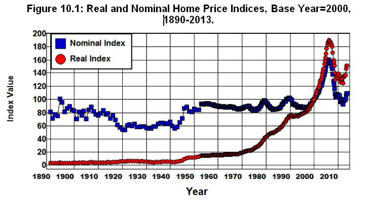
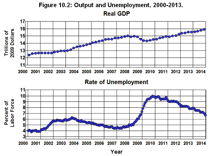
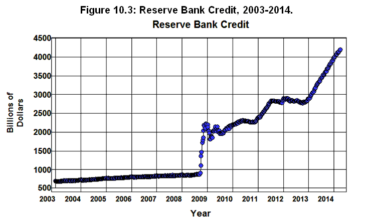
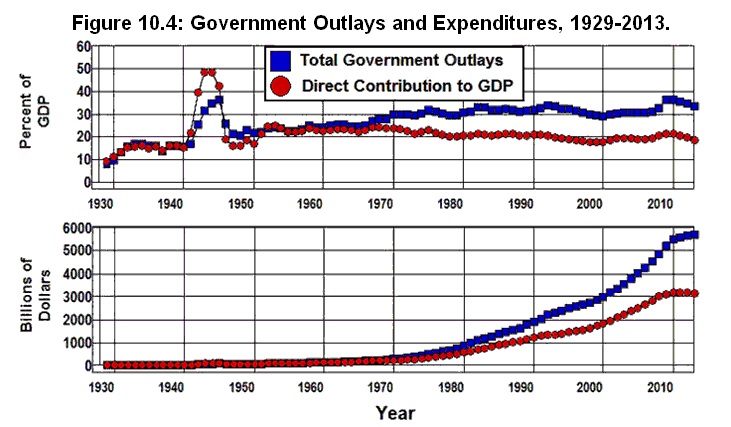
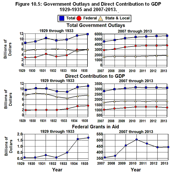
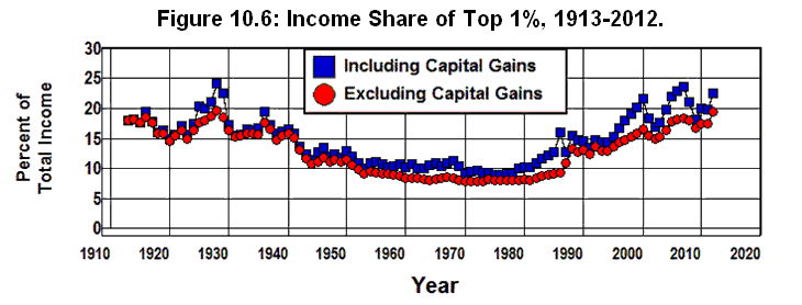
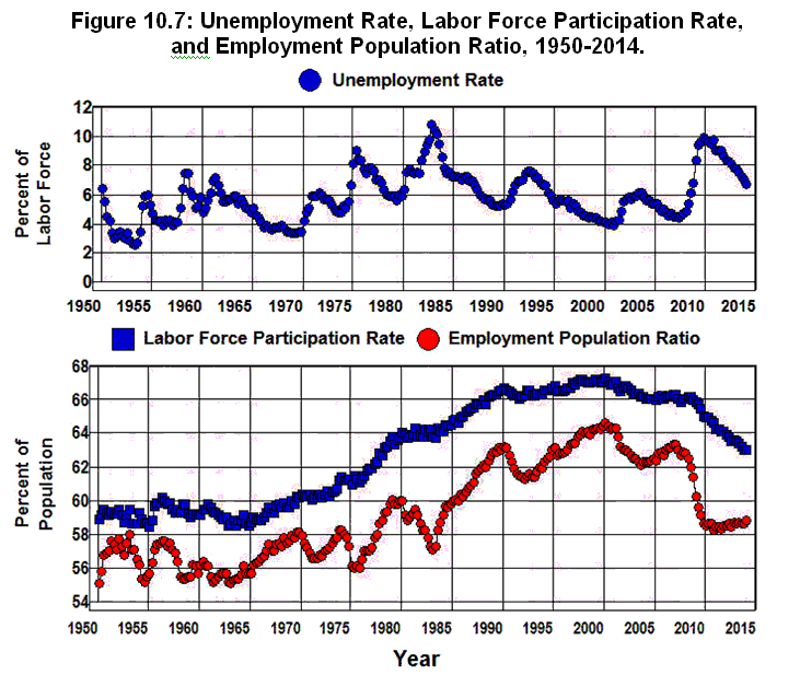
Where Did All The Money Go?
Chapter 11: History of the National Debt
George H. Blackford © 2010, last updated 5/16/2014
The federal deficit went from $74 billion in 1980 to $1.4 trillion 2009 while the Gross National Debt went from $735 billion in 1980 to $16.7 trillion at the end of 2013. These numbers are truly mystifying to those of us who have never had to worry about a million dollars let alone a billion or a trillion. The purpose of this chapter is to put these numbers in perspective and to give them concrete meaning in terms of the choices we face in dealing with our deficit/debt problems.
Concepts and Definitions
We begin with a few basic concepts and definitions.
The Federal Deficit and National Debt
The difference between the amount of money the government takes in from taxes and other sources of revenue (its receipts) and the amount it pays out in purchases of goods and services and other kinds of expenditures (its expenditures or outlays) is officially called the surplus. When the government takes in less than it pays out this difference is negative, and this negative surplus is the deficit. The relationships between government receipts, expenditures, and its surplus/deficits from 1901 through 2013 are shown in Figure 11.1, both in absolute amounts and as a percent of GDP.[11.1]
Source: Office of Management and Budget (1.1 1.2), Historical Statistics of the U.S. (Ca9-19)
As can be seen in this figure, whenever the government’s Receipts are greater than its Outlays the Surplus is positive, and there is no deficit. Similarly, whenever the government’s Receipts are less than its Outlays the Surplus is negative, and a deficit results.
Federal surpluses and deficits are related to the national debt in that when the government takes in less than it pays out it must borrow the difference (equal to the deficit) to finance its excess expenditures. As a result, whenever there is a deficit the national debt increases by (approximately) the amount of the deficit. Similarly, whenever the government takes in more than it pays out the resulting surplus is positive and is used to pay off the national debt. Thus, the national debt decreases by the amount of the surplus.[11.2]
One way of viewing the relationship between the national debt and the surplus/deficit is to think of the national debt as being the sum of all the deficits and surpluses the federal government has experienced since its inception. Figure 11.2 shows the total federal debt—commonly referred to as the national debt—from 1940 through 2013, both in terms of absolute dollars and as a percent of GDP. The federal debt is broken down into two categories:
The top line in Figure 11.2 plots the Gross National Debt, which includes all debt instruments issued by the federal government, including those held by federal agencies such as the Social Security Administration.
The bottom line in Figure 11.2 plots the Net National Debt, which is equal to gross debt less federal debt instruments held by federal agencies. Net National Debt is the portion of Gross National Debt held by the public, that is, by private individuals, businesses, financial institutions, and non-federal governmental institutions and agencies both foreign and domestic.
Source: Office of Management and Budget. (7.1)
At the end of 2013 Gross National Debt stood at $16.7 trillion and Net National Debt at $12.0 trillion. Of the $4.7 trillion difference, $2.7 trillion was held by the Social Security Administration in its Old-Age Survivors and Disability Insurance (OASDI) trust fund with another $0.3 trillion in its Medicare Hospital Insurance (HI) and Supplementary Medical Insurance (SMI) trust funds—a total of $3.0 trillion. Most of the remainder is held in the civil service and military retirement trust funds and the rest in the combined holdings of all other federal government agencies. Throughout this chapter the term “national debt” will refer to Net National Debt, unless designated otherwise.
Figure 11.1 is related to Figure 11.2 in that whenever the surplus is positive in Figure 11.1, the net federal debt shown in the top half of Figure 11.2 decreases by the amount of the surplus. Similarly, whenever the surplus is negative yielding a deficit in Figure 11.1, the net federal debt shown in Figure 11.2 increases by the amount of the deficit.[11.3]
Gross Domestic Product
The variables in the above figures are plotted both in terms of absolute values and as percentages of GDP. It should be obvious from looking at these figures that the absolute values do not tell us very much about the nature of the problems we are dealing with. Judging by the plots of absolute values it would appear that there was no national debt or deficit problem during World War II. Just the opposite was true, of course, as is made clear by the plots of these variables as a percent of GDP.
In attempting to understand the federal budget as it relates to the economic system as a whole it is essential that the numbers be examined in relative terms, that is, in relation to some other variable in the economy. There are a number of ways this can be done, but, for present purposes, I will use GDP as the point of reference, and the budget magnitudes will generally be expressed as a percent of GDP.
GDP—Gross Domestic Product as it is officially known—is the total value of all goods and services produced in the domestic economic system, and as such, it gives us a measure of the size of our economy. It also represents the total gross income created in the process producing domestic output in the economic system and is related to the total level of output produced as well as the total level of labor employed. When output, employment, and income increase GDP increases as well, and when output, employment, and income decrease GDP decreases.[11.4]
The importance of GDP in understanding the national debt arises from the fact that the national debt must be serviced—that is, the government must make both interest and principal payments on this debt. The ability of the government to service its debt without having to print money lies in its power to tax,[11.5] and since the main sources of the government’s tax revenue are from income and payroll taxes, the ratio of national debt to GDP gives a rough measure of the relationship between the government’s debt and the tax base available to service its debt. In general, increases in this ratio make it more difficult for the government to service its debt; decreases in this ratio make it easier for the government to service its debt.
As for the government’s receipts, outlays, and surplus, just as with the national debt, the ratios of these entities to GDP give a rough measure of their relationship to the tax base on which they ultimately depend, and, as such, these ratios play a crucial role in determining the government’s ability to finance its expenditures. In addition, changes in GDP have a direct effect on the level of government expenditures as well as on the level of tax receipts taken in by the government.
It is important to recognize that changes in the GDP will cause changes in government expenditures and receipts and, therefore, will also cause changes in the government's surplus or deficit and, thereby, its debt. An increase in GDP will automatically increase the amount of money taken in by the government in the form of income, payroll, and other taxes. At the same time, it will tend to decrease the level of government expenditures as unemployment compensation, welfare, food stamps, and other governmental assistance expenditures fall. By the same token, a fall in GDP will not only cause tax receipts to fall, but will cause government expenditures to increase as government assistance and other emergency expenditures increase.
Thus, a change in GDP will automatically affect the surplus or deficit as it affects government revenues and expenditures: An increase in GDP will automatically cause a surplus to increase or a deficit to decrease as tax receipts increase and expenditures fall; a decrease in GDP will automatically cause a surplus to decrease or a deficit to increase as tax receipts fall and expenditures increase.
The National Debt, 84 Years and Counting
The national debt stood at just 15.8% of GDP in 1929, but as a consequence of the Great Depression it rose to 42.8% by 1940.[11.6] Then came the deficits of World War II. As is indicated in Figure 11.1, government expenditures during the war were rather trivial by today’s standards in absolute terms, reaching a mere $92.7 billion in 1945. In relative terms, however, they were huge, amounting to 40.7% of GDP in 1944. At the same time, the deficit was also huge in relative terms, 26.9% of GDP in 1943. The same is true of the national debt shown in Figure 11.2 which grew to $271.0 billion for the gross debt and $241.9 billion for net debt by 1946. This amounted to 118.9% and 106.1% of GDP, respectively.
The United States was saddled with a huge debt burden at the end of the war as measured by the size of its net debt relative to GDP, a burden that was systematically reduced over the following 28 years. There were a few minor setbacks caused by the outbreak of the Korean War in 1950, the 1958 recession, and the confluence of a number of factors in the 1960s such as the Kennedy-Johnson tax cuts, the escalation of the Vietnam War, and Johnson’s declaration of war on poverty that caused net national debt as a percent of GDP to increase in 1968. Otherwise the fall in this ratio was virtually continuous from 1946 through 1974 as it went from 106.1% of GDP to 23.1%. After 1975, the debt ratio began to rise again, dramatically in the 1980s, but was brought under control again in the 1990s. Then in the 2000s it began to rise again and, as is apparent in Figure 11.2, exploded after 2007.
Falling Debt Burden from 1945 Through 1974
The federal budget was brought into balance fairly quickly after World War II, achieving a surplus in 1947, and though there were very few surpluses to follow, the budget was kept in fairly close balance from 1947 through 1974. As is shown in Figure 11.1, except for 1959 and 1968, the deficit was never greater than 2% of GDP.
The primary mechanism by which the budget was brought under control was, as will be shown in Chapter 12, by cutting defense expenditures as a percent of GDP as other components of the government grew. At the same time, much of the wartime tax structure was kept in place: The top marginal income tax rate ranged from 92% to 70% during this period. The top marginal corporate profits tax rate ranged from 53% to 48%, and the top marginal estate tax rate was 77%. This tax structure made it possible for the government to raise the requisite revenue as the economy adjusted to the war’s end and as government expenditures grew throughout the 1950s and 1960s.
A secondary factor that contributed to reducing the debt burden was the policies of the Federal Reserve and Treasury. The Treasury dominated the Federal Reserve during and immediately following the war, a situation that continued until the 1951 Federal Reserve-Treasury Accord that gave the Federal Reserve a certain degree of independence. (Bernanke) The Treasury’s low interest rate policy preceding the Accord led to a substantial increase in the supply of money. This, in turn, led to an effective annual rate of inflation of 5.6% from 1945 through 1951, and a 38.7% increase in the general level of prices was the result.[11.7]
In the presence of a relatively balanced budget, the inflation that resulted from the Treasury’s low interest rate policy contributed greatly to reducing the burden of the debt. Low interest rates made it possible for the Treasury to refinance its debt at minimal costs while the inflation increased GDP relative to the debt. The effect was to cause the net debt to GDP ratio to fall from 106.1% in 1945 to 65.5% in 1951. This 38.3% (40.6 percentage point) decrease in the debt to GDP ratio was accomplished in spite of the fact that the real output of goods and services produced during that period increased by only 4.3%[11.8] and the actual debt fell by only 11.4%.
The rate of inflation was brought under control after the Accord, and the effective annual rate of inflation was a modest 1.9% from 1952 through 1967, yet the debt to GDP ratio continued to fall throughout this period even though the government continued to experience deficits in its budget. The reason is that the production or goods and services increased dramatically.
From 1952 through 1967 the output of goods and services produced increased at an effective annual rate of 3.4%. This led to a 76.3% increase in total output by 1967, which combined with the 1.9% effective annual rate of inflation and the resulting 32.3% increase in prices, increased the nominal value of GDP by 134.3%. With a relatively balanced budget, the federal debt increased by only 24.2%. The result was a further fall in the debt to GDP ratio from 65.5% in 1951 to 31.8% by 1967. Thus, by 1967 the ratio of debt to GDP was below that of 1940, and the debt burden created by World War II had been completely eliminated along with half of the burden created by the Great Depression.[11.9]
The Kennedy-Johnson tax cuts combined with the escalation of the Vietnam War led to a deficit equal to 2.9% of GDP in 1968 that was converted into an 0.3% surplus in 1969 after the 1968 Revenue and Expenditure Control Act imposed a 10% income tax surcharge on individuals and corporations—the last surplus we were to see in the federal budget until 1998. The budget remained relatively balanced through 1974, and the debt ratio continued to fall with only a slight rise when the surcharge expired in 1970.
Debt Burden and the Great Inflation
The period from 1965 through 1984 is what Alan Meltzer has called The Great Inflation. As was noted above, from 1952 through 1967 the effective annual rate of inflation was 1.9%. From 1967 through 1982 it was 6.6% and from 1975 through 1981 it was 7.7%. Unlike the 1945-1951 inflation, this inflation contributed relatively little to reducing the debt burden.
The 1973 Arab oil embargo with its concomitant quadrupling of the price of oil caused the economy to falter. The resulting 1973-1975 recession with its increase in unemployment equal to 3.6% of the labor force caused the deficit to increase in 1975 to 3.4% of GDP and to 4.4% of GDP in 1976 as the debt to GDP ratio increased from 23.1% in 1974 to 27.1% by 1977. This ratio then fell somewhat by 1981 and stood at 25.5% in at the end of that year.
The reason the inflation of the 1970s had relatively little effect on reducing the debt burden is that inflation can increase GDP relative to the debt only if inflation increases GDP sufficiently to offset the rate at which the deficit increases the debt. That didn’t happen in the 1970s. In fact, the effect of the inflation on the deficit made the deficit worse than it otherwise would have been, especially in the aftermath of the inflation.
Changes in prices have the effect of transferring purchasing power—that is, wealth—between borrowers and lenders. When prices rise over the period of a loan the money that is lent can purchase more goods and services than the money that is paid back. As a result, inflation has the effect of transferring wealth from lenders to borrowers. Similarly, when prices decrease over the period of a loan the money that is lent can purchase fewer goods and services than the money that is paid back. As a result, deflation has the effect of transferring wealth from borrowers to lenders.
These transfers of wealth make the rate of interest at which people are willing to borrow or lend depend crucially on what they expect to happen to prices. Borrowers are less willing to borrow at high interest rates when they expect prices to fall and anticipate a loss in wealth from falling prices than when they expect prices to rise and anticipate a gain in wealth from increasing prices. The opposite is true for lenders. Lenders are more willing to lend at low interest rates when they expect prices to fall and anticipate a gain in wealth from falling prices than when they expect prices to increase and anticipation a loss in wealth from increasing prices. As a result, inflationary expectations tend to lead to high interest rates, and deflationary expectations tend to lead to low interest rates.
No one expected the inflation that followed World War II. The greatest fear at the time was of recession and falling prices as had been the case at the end of previous wars. World War II broke that pattern, and before anyone realized it the lack of inflationary expectations on the part of borrowers and lenders made it possible for the Federal Reserve to maintain low interest rates during the inflation of 1945 through 1951. As a result, the Treasury was able to finance its deficits and rollover[11.10] its debt without adding significantly to the deficit.
This was not the case during the Great Inflation with inflationary expectations rising throughout the period and remaining high into the 1990s. The effect of these rising and high expectations on interest rates can be seen in Figure 11.3 which shows the interest rates on various Treasury securities from 1941 through 2012.
Source: Economic Report of the President, 2012 (B73PDF|XLS),
Office of Management and Budget. (3.1)
The spike in interest rates from 1979 through 1982 was obviously caused by the tight monetary policy of the Federal Reserve during that period, but interest rates remained high from 1975 through 1990 even when the Fed’s monetary policy was not tight. From 1975 through 1990, federal deficits had to be financed and the debt rolled over at long-term interest rates above 7% and short-term rates above 4% and often above 6%.
The effect of having to rollover the debt at these exceptionally high interest rates is also shown in Figure 11.3 by the dramatic increase in interest paid by the federal government on the national debt as a percent of GDP from 1975 through 1995.
From 1981 to the Present
The national debt rose dramatically following 1980, reaching a peak as a percent of GDP of 47.8% in 1993. This dramatic increase in debt was precipitated by the
economic recession of 1981-1982 where unemployment increased by 3.8% of the labor force,
the 1981 Reagan tax cuts which led to a substantial loss in federal tax revenue, and
an increase in national defense expenditures from 4.8% of GDP in 1980 to 5.9% in 1987 during Reagan’s anti-Soviet defense buildup.
This increase in federal debt relative to GDP was eventually brought under control by 1995, in spite of the 1990-1991 recession that increased unemployment by 2.2% of the labor force. Net debt then fell as a percent of GDP from 1995 through 2000 as a result of
payroll tax increases that began in 1984,
the Clinton tax increases in 1993 along with eight other tax increases that were enacted following the 1981 tax cuts,
cuts in government expenditures from 1994 through 2000, mostly in defense, and
a dramatic increase in employment as the unemployment rate fell from 7.5% in 1992 to 4.0% in 2000.
By 2001, net federal debt stood at $3.3 trillion, which was just 31.4% of GDP compared to the peak of 47.8% it had reached in 1993. Then came the
2001 recession where unemployment increased by 2.0% of the labor force,
the 2001-2003 Bush II tax cuts which led to a substantial loss in federal tax revenue,
an increase in defense expenditures that accompanied the expansion of the war in Afghanistan into Iraq,
the bursting of the housing bubble in 2007 and the Great Crash of 2008 that led to the 2007-2009 recession where unemployment increased by 5.0% of the labor force,
Bush II's $152 Billion Economic Stimulus Act passed on February 13, 2008 to mitigate the effects of the economic downturn,
Bush II's $700 billion Troubled Asset Relief Program (TARP) passed on October 3 to bail out our financial institutions in the midst of the 2008 financial panic, and
Obama's $800 billion American Recovery and Reinvestment Act passed on February 17, 2009 to mitigate the effects of the financial crisis,
The net federal debt went from 31.4% of GDP in 2001 to 35.1% by 2007 as a result of the 2001 recession and 2001-2003 tax cuts. It then jumped to 39.3% of GDP in 2008, 52.3% in 2009, and had risen to 72.1% by the end of 2013. as a result of the financial crisis, ensuing depression, and the efforts made to stabilize the economy following the crisis. The debt itself went from $5.0 trillion in 2007 to $12.0 trillion in 2013 as a result of the recession and the government’s attempts to minimize its severity—a 140% increase in just 5 years. At the same time the budget went from a $236.2 billion surplus in 2000 to a $160.7 billion deficit in 2007, to a $458.6 billion deficit in 2008, a $1.4 trillion deficit in 2009, a $1.3 trillion deficit in 2010, and a $1.1 trillion deficit in 2012. By the end of 2013 the deficit had fallen to $679.5 billion..
Conclusion
It is apparent in looking at the history of the national debt that the primary sources of this debt are:
increases in defense expenditures associated with war.
economic downturns associated with recessions and depressions, and
cutting taxes in the face of rising government expenditures.
These conclusions will be reinforced when we look at the history of the federal budget in Chapter 12.
Appendix on Output, Prices, and Productivity
This Appendix elaborates on of some of the more technical aspects of measuring total output and the average price level. It also examines the relationship between changes in GDP, productivity, and employment.
Measuring Output
GDP is the total value of goods and serves produced in the domestic economy. This value is determined by multiplying the prices of goods and services produced by the quantities produced and summing to get their total value. This means that GDP will change when the prices of goods and services change even if the quantities produced do not change.
The levels of output and employment are related to the quantities of goods and services produced, not their values as such, and if we want a measure of total output that is related to employment and production we must adjust the nominal or money value of GDP for changes in prices. This is normally done by choosing the prices that exist at a particular point in time and using those prices to measure the value of the output of goods and serves produced at other points in time in order to make the measures comparable in terms of the quantities produced.
When the value of GDP is measured in this way the result is referred to as real GDP or GDP in constant prices, base year prices, or in base year dollars. Since real GDP is measured by holding prices constant, changes in real GDP can occur only if quantities change. Hence, real GDP gives us a way to measure changes in the sum of all the quantities of output produced.
Nominal GDP and real GDP measured in 2005 prices are plotted in Figure 11.4 from 1901 through 2010 using data from the Historical Statistics of the U.S. (Ca9-19) for the years 1901 through 1928 and from the Bureau of Economic Analysis (1.1.5) for the years 1929 through 2010. The values of nominal and real GDP in Figure 11.4 are, of course, the same in 2005 since that is the base year from which the prices were obtained.
Source: Bureau of Economic Analysis. (1.1.5) Historical Statistics of the U.S. (Ca9-19)
The nominal values of GDP are below the real values as measured in 2005 prices in the years preceding 2005 because prices in those years were, on average, lower than they were in 2005. As a result, the nominal values of GDP measured in current prices—that is, in prices that existed at the time—in those years overestimate the differences in the total quantity of output produced relative to that produced in 2005. Similarly, the nominal values of GDP are above the real values in the years following 2005 because prices in those years were, on average, higher than they were in 2005. As a result, the nominal values of GDP in those years underestimate the differences in total quantity of output produced relative to that produced in 2005.
The year to year rates of change in real GDP are also plotted in Figure 11.4. These rates of change give us a measure of the rate at which aggregate output (i.e., total output) changed from year to year.
Finally, it is worth noting that what we are doing here is adding apples and oranges, which everybody knows, you can't do. But, of course, you can add apples and oranges if you have a common unit of measurement, such as ponds or bushels. It is important to note, however, that when you do this you don't end up with either apples or oranges, but, rather, ponds or bushels of fruit, and the sum tells us nothing at all about the kind of fruit that is included in the result.
In measuring the total output within the economy, the common unit of measurement is the monetary unit, dollars, and the result of summing the various outputs of goods and services produced as measured in dollars is the total value of output produce: the 'real' value if prices are held constant over time or the current value if the prices that are current at the time are used. In either case, the sum tells us nothing at all about the composition of the total or how the composition changes over time. This apples and oranges problem is intrinsic in all aggregate measures (measures arrived at by adding to obtain a total) of disparate economic variables.
Measuring Prices
Since the difference between the value of nominal GDP and real GDP in each year is caused by the differences between current year prices and the prices that existed in the base year (2005 inFigure 11.4) if we divide nominal GDP by real GDP and multiply by 100 the result is a price index that expresses the weighted average (weighted by current year quantities produced) of current year prices to base year prices as a percent of base year prices. This index is called the implicit GDP deflator. A measure of the rate of inflation can be obtained from this index by calculating its year to year percentage changes.
The implicit GDP deflator in 2005 prices is plotted from 1900 through 2013 in Figure 11.5 using the GDP deflator implicit in the Historical Statistics of the U.S. (Ca9-19) for the years 1900 through 1928 and the series published by the Bureau of Economic Analysis (1.2.4.) for the years 1929 through 2013. The year to year percentages changes in this index that give the rate of inflation for each year in terms of the average price level as defined by the implicit GDP deflator are also plotted in this figure.
Source: Bureau of Economic Analysis. (1.1.5) Historical Statistics of the U.S. (Ca9-19)
Productivity
We can use real GDP as a measure of the output of goods and services produced in the economy, and by taking the year to year percentage change in this measure we can calculate the rate at which total output increases or decreases in each year. These rates are plotted in the bottom graph in Figure 11.4. They are important because the level of employment over time depends, in part, on the level of output. In general, an increase in output is associated with an increase in employment and a decrease in output is associated with a decrease in employment. However, the level of employment not only depends on the quantity of output produced, it also depends on the way in which output is produced.
The reason is that the amounts and kinds of tools and equipment and the ways things are done tend to increase and improve over time. These increases in the capital stock and improvements in technology tend to increase productivity which means they increase the amount of output a given number of workers can produce during a given amount of time. As a result, in order to maintain a given level of employment, real GDP must increase over time at the rate productivity increases. By the same token, in order to increase the level of employment, real GDP must increase at a rate that is greater than the rate at which productivity increases.
The Bureau of Labor Statistics’ productivity index of output per hour is plotted in Figure 11.6 from 1960 through 2008 along with the percentage changes in this index. The percentage changes in this index give the year to year rates at which productivity changed during each year. From 1960 through 2010 this index increased from 35.8 to 111.1—an increase of 210.3% which implies an effective annual rate of increase equal to 2.3%. This means that, over the past 50 years, real GDP had to increase, on average, by 2.3% per year just to maintain the level of employment that existed in 1960. It also means that during these 50 years it was necessary for output to grow, on average, by 2.3% plus the rate at which the labor force grew in order to keep the labor force fully employed.
Source: Economic Report of the President, 2013. (B49PDF|XLS)
Endnotes
[11.1] The Office of Management and Budget (OMB's) GDP data correspond to the federal government's fiscal year rather than the calendar year. Unfortunately, the OMB does not provide fiscal year estimates for years before 1930. I use the OMB's estimates for fiscal year GDP throughout this paper, except for the years before 1930. For the years before 1930 I use the mean of the current and previous calendar years' GDP from the Historical Statistics of the U.S. (Ca9-19) to estimate the fiscal year value of GDP. Using this methodology with the data from the Historical Statistics yields results that are identical, except for rounding error, to the fiscal year estimates of GDP given by the OMB for 1930 through 1947.
[11.2] This relationship is not exact in that the government can borrow money it doesn’t spend, thereby increasing the amount of cash it holds rather than pay down debt, and it can spend money in excess of its revenue without borrowing by reducing its holdings of cash. The government can also affect its cash/debt holdings by buying and selling assets that are, by definition, not included in its expenditures or revenue. See the Bureau of Economic Analysis's Table 3.2.
[11.3] See footnote 2 above.
[11.4] Some of the more technical concepts relating to GDP, employment, output, and income are explained in the Appendix on Output, Prices, and Productivity at the end of this chapter.
[11.5] The federal government also has the ability service its debt by printing money. The important of this fact is examined in Chapter 15. In the final analysis, however, it is the ability of the government to finance itself through taxes that makes economic stability possible, not the government's ability to print money. Attempting to finance the government by printing money without collecting the taxes needed to stabilize the monetary system inevitably leads to an increase in debt relative to GDP, hyperinflation, and a breakdown of the exchange system in the economy.
[11.6] The series on national debt published by OMB in Table 7.1 only goes back to 1940. The 1929 debt to GDP ratio reported above is calculated from Table B-1 and Table B-59 in the 1965 Economic Report of the President and is not strictly comparable to values published by the OMB and used throughout the rest of this paper. Aside from the calendar year/fiscal year difference discussed in footnote 1, the estimates of GDP have been refined since 1965, and the accounting conventions used to define and measure net and gross national debt have been refined as well. Neither number is the same today as it was in 1965. The 1940 debt ratio calculated from the GDP and Public debt at end of year values published in the 1965 ERP is 42.2% rather than the 43.6% published by the OMB today and reported above.
[11.7] These effective annual rates of inflation, as well as those that follow, are calculated from the 2005 base year GDP (chained) Price Index published by OMB in Table 10.1. The effective annual rates used throughout this paper are calculated from the compound interest formula:
Pn = P0 x ∏(1 + r)i,
where
i = 0, 1, 2,. . .,n,
P0 is the starting principle,
Pn is the ending principle, and
r is the effective annual rate.
This formula assumes annual rather than continuous compounding.
[11.8] This value was computed by deflating OMB’s fiscal year GDP in Table 10.1 by the 2005 base year GDP (chained) Price Index in this table and calculating the percentage change in the resulting real value of GDP measured in 2005 prices from 1945 through 1951. Changes in output will be measured in this way in what follows.
[11.9] The debt ratio fell below the 1940 level in 1962.
[11.10] Approximately one third of the national debt is in the form of Treasury bills that mature in less than one year and one half is in the form of Treasury notes that mature in less than ten years. (B87PDF-XLS) When there is a deficit in the federal budget, the debt obligations of the government must be paid when they come due by the government issuing new debt instruments in order to obtain the cash necessary to pay off the old debt instruments—that is, the Treasury must rollover its debt.
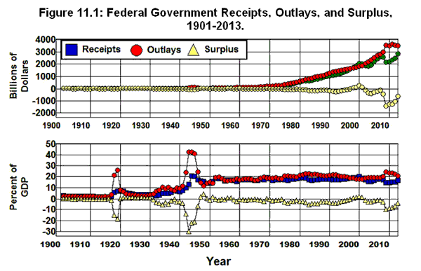
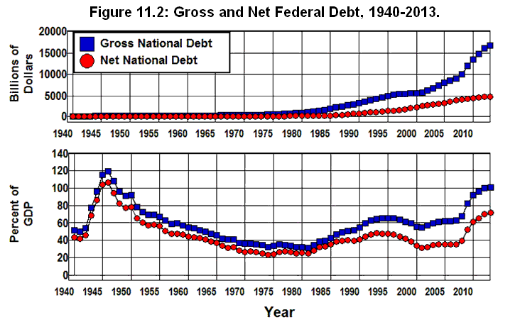
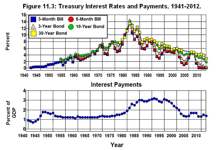
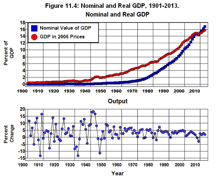
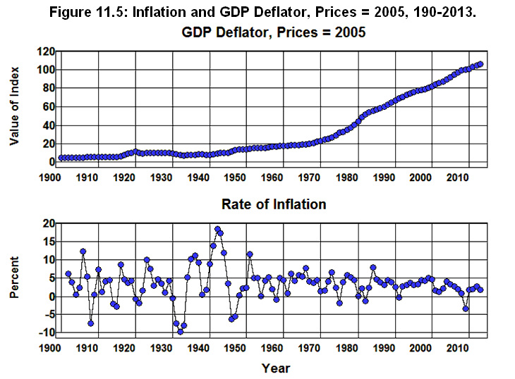
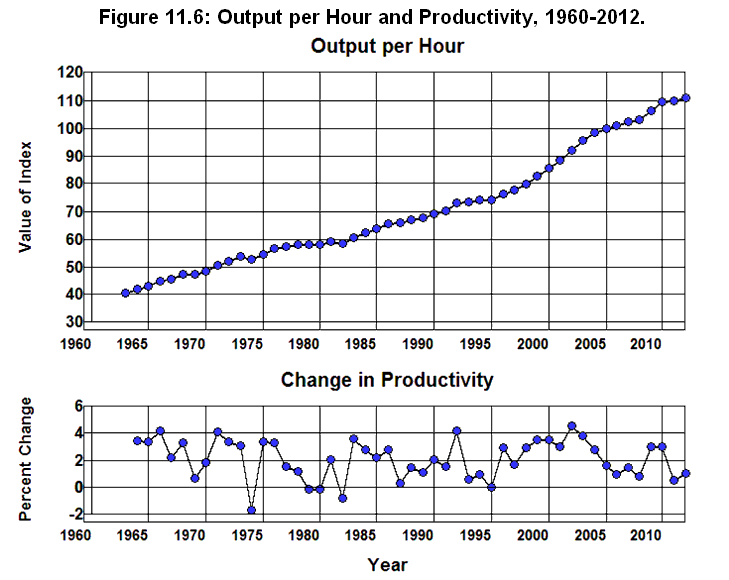
Chapter 12: History of the Federal Budget
George H. Blackford © 2010, last updated 5/4/2014
It is very difficult, if not impossible, to understand how the federal budget got to where it is today without examining how our country has changed since 1929. The Crash of 1929, the economic catastrophe of the Great Depression, the devastation of World War II, and the Cold War that followed had profound effects on the American psyche. We are not the same country we were in 1929, and this is particularly so when it comes to how we view government. (Kennedy)
As was noted in Chapter 4 and Chapter 5, prior to 1929, most of our political leaders and much of the American public had an unbridled faith in the magical powers of free-market capitalism. The catastrophe of the Great Depression shook that faith and changed us from a country that saw the primary role of government as serving the needs of the plutocracy to a country that sees the primary role of government as serving the needs of ordinary people. This led to the federal government sponsoring social-insurance programs such as Social Security, Unemployment Compensation, the Farm Program, Aid to Dependent Children, Medicare, Medicaid, and Supplemental Security Income that did not exist at the federal level before the Great Depression. (Kennedy)
In addition, before 1929 we were an isolationist country, reluctant to intervene in the domestic affairs of other countries except, of course, in Latin America. The devastation of World War II, combined with the Cold War that followed, shook our faith in isolationism and changed us from an isolationist country focused on Latin America into one willing to intervene in the domestic affairs of countries throughout the world. This led to a tremendous emphasis on national defense following World War II and to a peacetime military far beyond anything we had experienced previously. (Kennedy)
These two factors—the loss of faith in free-market capitalism brought on by the Great Depression and our national interventionist policies brought on by World War II and the ensuing Cold War—have had profound effects on the nature of our federal government, and, in particular, on the size of its budget.
Government Expenditures
The dramatic effect the Great Depression, World War II, and the Cold War had on the size of the federal budget can be seen in Figure 12.1 which plots total government outlays as a percent of GDP from 1901 through 2013.
Source: Office of Management and Budget (1.1 10.1),Historical Statistics of the U.S. (Ca9-19) [12.1]
As is shown in this figure, since the end of the Korean War (1953) the federal government has been 5 to 8 time larger than it was back in 1929.
Federal government outlays were 3.1% of GDP in 1929. Then came the Great Depression of the 1930s. By 1941 total outlays had increased to 11.7% of GDP. Next came the dramatic increases in government outlays from 1942 through 1947 during World War II and the subsequent occupation of the Axis countries following the war. Total outlays fell to 11.3% of GDP by 1948 as we demobilized from the war. This was below the 1941 level, but still more than three times the size of the federal government relative to the economy that existed in 1929. Then came the Cold War.
The Cold War began in earnest on June 27, 1948 when the Soviet Union cut all surface traffic to West Berlin. This led to the Berlin Airlift and the European Recovery Act—commonly referred to as the Marshall Plan—was enacted later that year. That same year the Soviet Union detonated its first nuclear bomb, and the Communists drove the Nationalists from the mainland in China. The Korean War began on June 25,1950 when North Korean troops crossed the border with South Korea, and the first U.S ground combat troops arrived in Korea on July 1st of that year. By the time that war had ended in 1953 federal government outlays had increased to 19.9% of GDP—a 75% increase over 1948—and the federal government was never to see its prewar low again.
From the end of the Korean War through 2008, the federal government fluctuated between the 1956 low of 16.1% of GDP and a 1983 high of 22.8%. By 2000, the size of the federal budget had fallen to 17.6% of GDP—23% below its 1983 high, 17% below where the federal government was in 1980, and comparable in size to the government in the early 1960s before the Viet Nam defense buildup that began in 1965.
After the military buildup for the Iraq and Afghan wars and before the crash in 2008, the budget was back to 19% of GDP but still 17% below what it was in 1983, 10% below where it was in 1980. Then came the Crash of 2008, after which the budget grew to a high of 24.4% of GDP by 2009 as a result of the ensuing economic crisis and then fell back to 20.8% by 2013 which was about where it was in 1980.
But in looking at the history of this period, it is clear that out interventionist policies were not the only factors that contributed to the increase in the federal budget following the Great Depression and World War II. As can be seen in Figure 12.2, which gives a breakdown or the federal budget by Superfunction from 1940 through 2013, the rise in social-insurance programs (Human Resources) also played a dramatic role in this increase.
Source: Office of Management and Budget. (3.1 10.1)
It is clear from this figure that while Defense dominated the federal budget during and immediately following World War II, Human Resources have played a dominant role in the federal budget following the end of the Korean War in 1953.
National Defense
Figure 12.3 plots defense expenditures as a percent of GDP and of the federal budget from 1940 through 2013.
Source: Office of Management and Budget. (3.1 10.1)
The role that defense expenditures played in increasing the size of the federal government after World War II is clearly indicated in this figure. National Defense stood at 1.7% of GDP and 17.5% of the budget in 1940 before the war. After reaching 37% of GDP% and 89% of the budget during the war it had fallen back to 3.5% of GDP and 30.6% of the budget by 1948. By the end of the Korean War defense expenditures were back up to 13.8% of GDP and 69.4% of the budget. National Defense then gradually declined to 7.1% and 42.8% by 1965. Then came Vietnam.
National Defense reached a peak during the Vietnam War in 1968 at 9.1% of GDP and 46.0% of the budget and then declined gradually through the era of Détente, reaching a low of 4.5% of GDP and 23.1% of the budget in 1979. Then came the Reagan anti-Soviet defense buildup which increased defense expenditures to 6.0% of GDP and 27.6% of the budget by 1986. Defense expenditure gradually fell relative to the economy and the budget following 1986 until they reached a post World War II low of 2.9% of GDP and 16.4% of the budget in 2001. Defense expenditures then rose again following the 9/11 attack in response to the Afghanistan and Iraq wars reaching a peak in 2010 at 4.7% of GDP and 20.1% of the budget. By 2013 Defense stood a 3.8% of GDP and 18.3% of the budget.
Outlays for Nation Defense in 2013 were substantially below their levels during the Cold War era, but were about where they stood in the early 1990s at the end of the Cold War. They were also more than twice the 1.7% of GDP they were in 1940 before World War II and greater as a percent of GDP than the entire federal budget in 1929.
While dominating the federal budget in the early post World War II years, the importance of National Defense has declined dramatically over the past 60 years both as a percent of GDP and of the federal budget. As a result, this component of the budget shares relatively little responsibility for the 15% to 18% of GDP increase in government outlays since 1929—as little as 2% or 3% of GDP. But as defense expenditures declined over the past 60 years, the social-insurance programs that grew out of the New Deal expanded. This tradeoff is quite obvious in Figure 12.2 as indicated by the dramatic decrease in the Defense component of the budget and the dramatic increase in the Human Resources component in this figure.
Human Resources
As was noted above, the Human Resources category of the federal budget is where the our social-insurance programs are to be found. The largest component in this category, as broken down in the official statistics, is Social Security followed by Income Security, Medicare, Health, Veterans Benefits, and Education & Social Services. Income Security includes such things as General retirement and disability insurance, Federal employee retirement and disability, Unemployment compensation, Housing assistance, and Food and nutrition assistance. The programs that fall under the heading of Human Resources in the federal budget are examined in detail in Chapter 13 and Chapter 14 below, but a breakdown of this category of the federal budget by its major components is given in Figure 12.4.
Source: Office of Management and Budget. (3.1 10.1)
There are three things worth noting about the Human Resources category of the budget:
The Social Security and Income Security programs that begun during the New Deal grew systematically until they reached their maturity in the 1980s. These components of Human Resources then leveled off at roughly 4.5% and 3% of GDP, respectively, as they grew to roughly 22% and 15% of the budget. (The spike in Income Security following 2007 is clearly the result of the recession that began in that year.) These two items in the budget are expected to increase gradually until 2035 as the baby boomers retire and then decrease somewhat from then on.
Veterans Benefits and Education & Social Services are a relatively insignificant portion of this category of the budget, and of the budget itself. Each comprises less than 1% of GDP and less than 5% of the budget. In addition, both of these items have been cut substantially since 1980, and there is no reason to believe that much can be gained from further cuts in these components of the budget in dealing with the deficit/debt problem.
While both Social Security and Income Security peaked in 1980 and had fallen by 2007, both the Medicare and Health components of the budget have trended upward since 1965 and there is little indication that this trend will not continue in the future. Even though Social Security and Income Security are the largest single components of Human Resource today, they have been less than the sum of Medicare and Health since 2004. While Social Security and Income Security are both expected to increase in the future, the increases in these two components is predictable in a way that the increases in Medicare and Health are not.
Social Security increased by 1.7% of GDP from 1965 through 2007 and is expected to increase by an additional 2.0% by 2035. The sum of Medicare and Health increased by 4.6% of GDP over the same period, and there is no way of knowing what will happen to this sum in the future. It is the rise in healthcare costs that presents the greatest challenge in the future when it comes to managing the federal budget, not Social Security or Income Security.
Net Interest
Net Interest is interest paid by the federal government net of the interest paid within the government. In other words, it is the interest paid on the Net National Debt. Net Interest is plotted in Figure 12.5.
Source: Office of Management and Budget. (3.1 10.1)
This category increased dramatically in the 1980s. It reached a peak in 1991 at 3.2% of GDP and 14.7% of the budget—dramatically above its 1959 post-war low of 1.1% of GDP and 6.3% of the budget—and subsequently fell to a low of 1.3% of GDP and 7.0% of the budget in 2004 prior to the crash in 2008 and was at 1.3% of GDP and 6.4% of the budget in 2013.
Physical Resources
A breakdown of the Physical Resources category of the federal budget is given in Figure 12.6. This category consists of Transportation, Natural Resources and Environment, Energy, Commerce and Housing Credit, and Community and Regional Development.
Source: Office of Management and Budget. (3.1 10.1)
None of the items in the Physical Resources portion of the budget have exceeded 1% of GDP since 1950 except Commerce & Housing (which includes the FDIC and other federal depository insurance programs) and only Transportation has exceeded 3% of the budget in the past 60 years. Aside from the fact that these programs take up a rather insignificant portion of the federal budget and play a vital role in the functioning of our economic system, all of these programs have been cut substantially since 1980, and there is no reason to believe that much can be gained from further cuts in these components of the budget in dealing with the deficit.
All Other Government Functions
Finally, we get to All Other Government Functions. A breakdown of this category is presented in Figure 12.7. It includes International Affairs, Science and Technology, Agriculture, Administration of Justice, General Government, and Undistributed Offsetting Receipts.[12.2]
Source: Office of Management and Budget. (3.1 10.1)
Even though these functions of the federal government play a vital role in the functioning of our society and of our economic system, each of these functions represents a very small part of GDP and of the federal budget. Since 1990, none have exceeded 0.4% of GDP or 2% of the budget and most hover around 0.2% of GDP and 1% of the budget. International Affairs,[12.3] Agriculture, Science and Technology, and General Government have all been cut substantially since 1980. Only Administration of Justice has increased since 1980 and has, in fact, increased fivefold since 1950 as a percent of our economy—mostly as a result of the war on drugs that began in the Nixon administration and has been fought ever so valiantly at ever greater expense since then.
Government Revenues
Next we look at the revenue side of the budget. Figure 12.8 shows the total federal revenue as a Percent of GDP from 1901 through 2013.[12.4]
Source: Office of Management and Budget. (1.1 10.1) Bureau of Economic Analysis. (1.1.5)
The dramatic effect the Great Depression, World War II, and the Cold War had on the size of the federal government can be seen in this figure as well as in the plot of federal outlays in Figure 12.1. Total federal revenue stood at 3.8% of GDP in 1929. Then came the Great Depression of the 1930s, and by 1941 total revenue had increased to 7.5% of GDP. After the dramatic increase to 20.5% during the war, it receded to a post war low of 14.1% of GDP in 1950—a level that was never to be seen again. After 1950, total federal revenue reached a high of 19.9% of GDP in 2000 and a low of 14.6% in 2009.
Figure 12.9 gives a breakdown of the various sources of federal revenue from 1934 through 2013.
Source: Office of Management and Budget. (2.3 10.1)
It is clear from this figure not only that the level of federal revenue has increased dramatically since 1934, but that the way in which the federal government is financed has changed dramatically as well.
Federal Income Taxes
Prior to World War II, the largest source of federal revenue was federal excise taxes. During the war, personal and corporate income taxes took center stage. In 1934, Personal Income Tax receipts were 14.2% of total federal revenues. In 1950 they were 40%—only 5 percentage points below the World War II peak of 45.%. They then fluctuated between 41% and 47% of total revenues until 1969—hitting a low of 41.3% of revenues in 1967 after the Kennedy-Johnson tax cut and rebounding to 46.7% in1969 in response to the 10% surcharge passed in 1968. In 1970, Personal Income Tax receipts rose to 46.9% of total receipts.
Personal Income Tax receipts then declined to a low of 43.9% of revenue by 1975 as the income tax surcharge expired in 1970 and as a result of the 1973-1975 recession. Receipts from this source began to rise again in 1977 as we pulled out of the recession and as the rampant inflation of the late 1970s moved people into higher tax brackets. It reached a peak of 8.6% of GDP and 48% of total revenues during the 1981-1982 recession and before the 1982 Reagan tax cuts. This feat was accomplished in spite of the fact that 6 of the 9 major tax bills enacted between 1968 and 1981 reduced federal revenue.
The Reagan tax cuts lowered Personal Income Tax receipts from 47.7% of total revenue in 1981 to 44.8% by 1984. They stood at 43.2% in 1995. In that year the economy was growing quite rapidly and the 1993 Clinton tax increases—along with the 8 other tax bills enacted since 1982 that increase federal revenues—were beginning to take hold. Personal Income Tax receipts continued to rise after the Clinton tax increase until they hit an all time high of 9.5% of GDP in 2000 and 49.9% of federal revenues in 2001.
Then came the 2001-2002 recession and the 2001-2003 Bush Tax Cuts. As a result, revenue from this source fell to 6.3% of GDP by 2004 and to 43.0% of federal revenues. Income tax receipts climbed back up to 45.3% of federal revenues in 2007, in spite of the Bush tax cuts, as the economy recovered from the recession and the housing boom and profits in the financial sector reached their peak. Then the housing bubble burst, and the economy imploded. By 2010 income tax receipts were at their lowest level since 1950—5.8% of GDP and 41.6% of total federal receipts.
By 2013 the revenue from the personal income tax had reached 7.9% of GDP and 47.4% of total receipts primarily as a result of the spending cuts and the rescission of portions of the 2001-2003 Bush Tax Cuts mandated by the Budget Control Act of 2011.
Corporate Taxes
Corporate Income Tax receipts were less than 1% of GDP in 1934 and amounted to 12.3% of total federal revenue. They then rose to 5.9% of GDP and 32.1% of federal revenue by 1952 and declined to 2.0% of GDP and 10.2% of revenue by 2000. In 2013 Corporate Income Tax receipts were 1.7% of GDP and 9.9% of total federal revenue. As we will see in Chapter 17, the loss of revenue from this source has had a detrimental effect on the economy.
Payroll Taxes
Payroll Tax receipts have increased consistently since 1934 as the Social Security Systems matured. They reached a peak in 2001 at 6.4% of GDP.
As is clear from Figure 12.9, payroll taxes have played a major role in financing the increase in the federal budget since 1934 going from virtually nothing in that year to a high of 42.3% of total federal revenue in 20049. Not only have payroll taxes financed Social Security’s retirement and disability and Medicare’s Part A programs from their inception since 1984, payroll taxes have contributed some $3.0 trillion to the federal government’s general fund as the Social Security Administration built up the OASDI and Medicare trust funds by this amount. The significance of this buildup is examined in Chapter 17.
Federal Excise Taxes
Excise taxes are taxes on specific goods or services, such as taxes on tobacco, alcohol, and gasoline. Their importance in funding the federal government has declined steadily since the 1930s when they comprised 2.2% of GDP and 45.8% of total receipts in 1934. In 2013 they amounted to only 0.5% of GDP and 3.0% of federal revenue.
All Other Sources
Other sources of federal revenue have been relatively insignificant since the 1930s. They consist of such things as the Estate and Gift Taxes, Customs Duties, and Federal Reserve Earnings. At their peak during the past seventy years their sum has barely exceeded 1% of GDP, and they have provided approximately 5% of total federal revenue since 1960. They stood at 0.87% of GDP in 2000, before the Bush tax cuts. They were down to 0.59% by 2005. Because of the enhanced earnings that have resulted from the extraordinary actions taken by the Federal Reserve during the current crisis, the total of all other sources of federal revenue reached 0.92% of GDP in 2013, and amounted to 5.5% of federal revenues in that year. A breakdown of this category from 1940 through 2013 is plotted in Figure 12.10.
Source: Office of Management and Budget. (2.5 10.1)
Summary
The expenditure and revenue sides of the budget from 1940 through 2013 are summarized in Figure 12.11.
Source: Office of Management and Budget. (3.1 2.1 10.1)
It is clear from the graphs in this figure that the major components on the expenditure side of the budget today lie in the Human Resources category of the budget—Social Security, Income Security, Health, and Medicare.
It is also clear from the graphs in this figure that the primary mechanisms by which the increase in the Human Resources category of the budget has been financed over the past 60 years is through decreasing expenditures for National Defense and increasing payroll taxes as a percent of GDP. This decrease in National Defense and increase in payroll taxes was used to finance a reduction in the Corporate Tax and all other taxes collected by the federal government as well. The reduction of taxes on corporations has been especially dramatic in this regard.
Finally, it is clear from Figure 12.11 that if we are to have less government the place we must cut the budget is in Human Resources and possibly Defense. Virtually everything else has been cut to the bone since 1980. In fact, by 1913, All Other Outlays relative to the size of the economy (3.1% of GDP) was below where it had been at any point during the previous seventy-three years. This has occurred in spite of obvious need for growth in the Transportation, Natural Resources and Environment, Energy, Commerce and Housing Credit, Community and Regional Development, International Affairs, Science and Technology, Agriculture, Administration of Justice, and General Government functions of the federal government as our population has grown and become more urbanized, our role in the world has become more complicated, and and our economic system has faltered as a result of the government's inability to perform the basic functions that it must perform in these areas if we are to prosper.
As was noted above, the Human Resources portion of the budget is made up of the social-insurance programs that have grown out of Roosevelt's New Deal. Given the importance of these programs in the current debate over debt reduction and the size of government, it is worth looking at the history of our social-insurance programs in detail. We will do this in the next two chapters.
Appendix on the Federal Budget in 2013
Table 12.1 gives the expenditures in each functional and subfunctional category in the Office of Management and Budget’s Table 3.2—Outlays by Function and Subfunction along with the percent of GDP and of the outlays allocated to each category in 2013.
Table 12.1: Breakdown of Federal Budget by Function and Subfunction, 2013.
OMB's Table 3.2—OUTLAYS BY FUNCTION AND SUBFUNCTION: 2013 Function and Subfunction (Billions of Dollars) Billions of Dollars Percent of GDP Percent of Budget 050 National Defense: 633.4
3.81% 18.33% 051 Department of Defense-Military: 607.8 3.66% 17.59% Military Personnel 150.8 0.91% 4.37% Operation and Maintenance 259.7 1.56% 7.52% Procurement 114.9 0.69% 3.33% Research, Development, Test, and Evaluation 66.9 0.40% 1.94% Military Construction 12.3 0.07% 0.36% Family Housing 1.8 0.01% 0.05% Other 1.4 0.01% 0.04% 053 Atomic energy defense activities 17.6 0.11% 0.51% 054 Defense-related activities: 8.0 0.05% 0.23% 150 International Affairs: 46.4 0.28% 1.34% 151 International development and humanitarian assistance 22.8 0.14% 0.66% 152 International security assistance 9.9 0.06% 0.29% 153 Conduct of foreign affairs 13.0 0.08% 0.38% 154 Foreign information and exchange activities 1.5 0.01% 0.04% 155 International financial programs -0.8 -0.01% -0.02% 250 General Science, Space, and Technology: 28.9 0.17% 0.84% 251 General science and basic research 12.5 0.08% 0.36% 252 Space flight, research, and supporting activities 16.4 0.10% 0.48% 270 Energy: 11.0 0.07% 0.32% 271 Energy supply 9.0 0.05% 0.26% 272 Energy conservation 1.2 0.01% 0.04% 274 Emergency energy preparedness 0.2 0.00% 0.01% 276 Energy information, policy, and regulation 0.5 0.00% 0.02% 300 Natural Resources and Environment: 38.1 0.23% 1.10% 301 Water resources 7.7 0.05% 0.22% 302 Conservation and land management 10.7 0.06% 0.31% 303 Recreational resources 3.5 0.02% 0.10% 304 Pollution control and abatement 9.6 0.06% 0.28% 306 Other natural resources 6.6 0.04% 0.19% 350 Agriculture: 29.5 0.18% 0.85% 351 Farm income stabilization 25.0 0.15% 0.73% 352 Agricultural research and services 4.4 0.03% 0.13% 370 Commerce and Housing Credit: -83.2 -0.50% -2.41% 371 Mortgage credit -87.9 -0.53% -2.54% 372 Postal service -1.8 -0.01% -0.05% 373 Deposit insurance 4.3 0.03% 0.12% 376 Other advancement of commerce 2.2 0.01% 0.06% 400 Transportation: 91.7 0.55% 2.65% 401 Ground transportation 60.0 0.36% 1.74% 402 Air transportation 21.5 0.13% 0.62% 403 Water transportation 9.8 0.06% 0.28% 407 Other transportation 0.4 0.00% 0.01% 450 Community and Regional Development: 32.3 0.19% 0.94% 451 Community development 7.8 0.05% 0.23% 452 Area and regional development 1.5 0.01% 0.04% 453 Disaster relief and insurance 23.0 0.14% 0.67% 500 Education, Training, Employment, and Social Services: 72.8 0.44% 2.11% 501 Elementary, secondary, and vocational education 42.4 0.26% 1.23% 502 Higher education -0.5 0.00% -0.02% 503 Research and general education aids 3.7 0.02% 0.11% 504 Training and employment 7.3 0.04% 0.21% 505 Other labor services 1.9 0.01% 0.05% 506 Social services 18.1 0.11% 0.52% 550 Health: 358.3 2.16% 10.37% 551 Health care services 321.8 1.94% 9.32% 552 Health research and training 32.9 0.20% 0.95% 554 Consumer and occupational health and safety 3.6 0.02% 0.10% 570 Medicare: 497.8 3.00% 14.41% 600 Income Security: 536.5 3.23% 15.53% 601 General retirement and disability insurance 7.0 0.04% 0.20% 602 Federal employee retirement and disability 131.7 0.79% 3.81% 603 Unemployment compensation 70.7 0.43% 2.05% 604 Housing assistance 46.7 0.28% 1.35% 605 Food and nutrition assistance 109.7 0.66% 3.18% 609 Other income security 170.7 1.03% 4.94% 650 Social Security: 813.6 4.90% 23.55% 700 Veterans Benefits and Services: 138.9 0.84% 4.02% 701 Income security for veterans 65.9 0.40% 1.91% 702 Veterans education, training, and rehabilitation 12.9 0.08% 0.37% 703 Hospital and medical care for veterans 52.5 0.32% 1.52% 704 Veterans housing 1.3 0.01% 0.04% 705 Other veterans benefits and services 6.3 0.04% 0.18% 750 Administration of Justice: 52.6 0.32% 1.52% 751 Federal law enforcement activities 27.3 0.16% 0.79% 752 Federal litigative and judicial activities 14.6 0.09% 0.42% 753 Federal correctional activities 6.9 0.04% 0.20% 754 Criminal justice assistance 3.8 0.02% 0.11% 800 General Government: 27.8 0.17% 0.80% 801 Legislative functions 3.7 0.02% 0.11% 802 Executive direction and management 0.5 0.00% 0.01% 803 Central fiscal operations 12.1 0.07% 0.35% 804 General property and records management 0.0 0.00% 0.00% 805 Central personnel management 0.4 0.00% 0.01% 806 General purpose fiscal assistance 7.9 0.05% 0.23% 808 Other general government 6.0 0.04% 0.17% 809 Deductions for offsetting receipts -2.7 -0.02% -0.08% 900 Net Interest: 220.9 1.33% 6.39% 950 Undistributed Offsetting Receipts: -92.8 -0.56% -2.69% Total outlays 3,454.6 20.79% 100.00% Source: Office of Management and Budget (3.2 10.1)
Footnotes
[12.1] See Chapter 11, footnote 1 for an explanation of the construction of this graph.
[12.2] The federal government takes in money other than through taxes in the form of fees and other payments. These payments often arise from businesslike transactions with the public (fees collected by the FDIC for deposit insurance, for example) and are referred to as offsetting receipts in the federal budget. In most cases they are assigned to the specific functional category in which they arise, and are treated as a negative expenditure within that functional category rather than as a source of revenue or a receipt that is available to the rest of the government. As a result, the outlays that appear in the individual functional categories of the budget indicate the governmental resources allocated to that category net of the resources received in that category through market mechanisms.
There are some sources of non-tax receipts that do not arise from businesslike transactions with the government (payments by Federal agencies to employee retirement funds, for example) or that do arise from businesslike transactions with the government but are so large that they would distort the functional totals if they were assigned to the functional category in which they arise (payments on federal oil and gas leases, for example). These payments are not assigned to a particular functional category in the budget, and are referred to as undistributed offsetting receipts. They represent funds that are available to the general fund to be distributed throughout the budget. As a result, these funds are treated as a negative outlay in the federal budget, rather than as a revenue, and these negative outlays are added in as a separate item in order to arrive at total outlays. (See: UNDISTRIBUTED OFFSETTING RECEIPTS.)
Undistributed offsetting receipts reached a high of 1.1% of GDP and 6.2% of the budget in 1974 and a low of 0.4% of GDP and 1.1% of the budget in 1999 through 2002. This category of the budget has averaged 0.7% of GDP and 3.3% of the budget since 1970 and stood at 0.6% of GDP and 2.7% of the budget in 2013.
[12.3] It is, perhaps, worth noting that less than half of the International Affairs budget is devoted to humanitarian foreign aid. The rest funds the operations of our foreign embassies and provides for military and law enforcement assistance to foreign governments. A breakdown of the federal budget by Function and Subfunction in 2013 (OMB's Table 3.2—Outlays by Function and Subfunction: 1962–2019) along with the percent of GDP and of the federal budget that each program represented in that year is given in the Appendix on the Federal Budget in 2013 at the end of this chapter.
[12.4] See footnote 2 above.
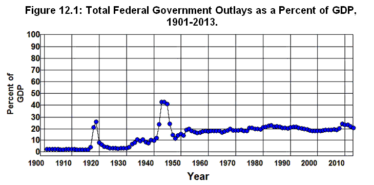
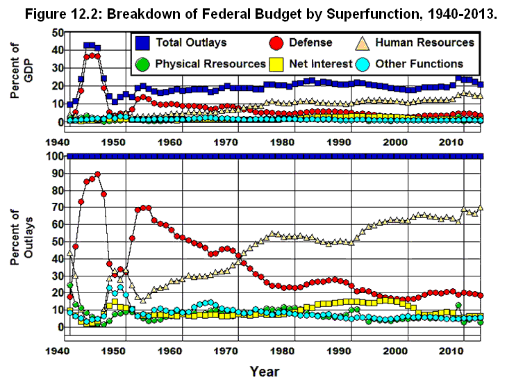
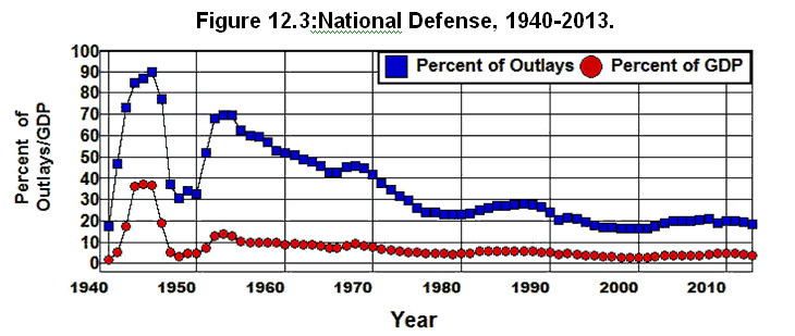

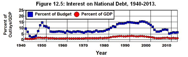
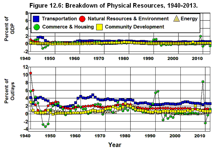
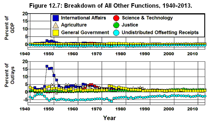
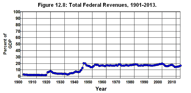
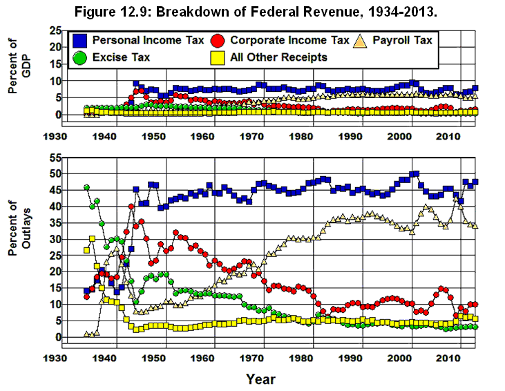
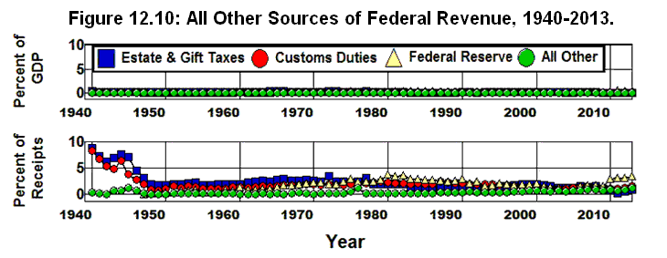
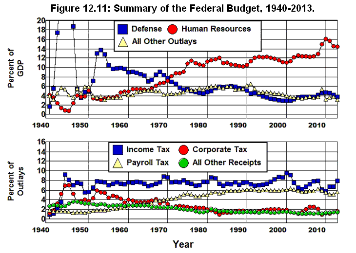
Chapter 13: Human Resources and Social Insurance
George H. Blackford © 2010, last updated 5/4/2014
As we saw in Chapter 12, the largest increase in the federal budget over the past sixty years has been in the area of Human Resources. This category went from 33.4% of the budget and 5.1% of GDP in 1950 to 64.4% of the budget and 12.3% of GDP in 2007.[13.1] The great bulk of the expenditures in this category fund our social-insurance programs. These are the programs—the largest of which are Social Security and Medicare—that grew out of Franklin D. Roosevelt’s New Deal.
Social Security and Medicare, as well as many other programs provided by the federal government, are insurance programs in that they provide protection against the possibility of becoming indigent as a result of a devastating loss that may or may not occur. Social Security, for example, provides insurance against the possibility of not being able to save enough to provide for one's retirement, the loss of one's savings as a result of poor investment choices, outliving one's savings, or the inability to earn a living as a result of becoming disabled or through the premature death of a working parent or spouse. Medicare provides insurance against the possibility of becoming uninsurable due to poor health in one's elder years and the inability to meet one's healthcare needs out of savings.
These are social-insurance programs in that they pool the risk across all or most members of society by including all or most members of society in the payment and benefit structure they offer. In addition, they provide the kind of insurance that cannot be provided by private insurance companies in that there exists no market mechanism by which these kinds of risk can be efficiently or effectively pooled within the economic system in the absence of government intervention.
Payments for Individuals
Most of the expenditures in the Human Resources category of the budget are included in the Office of Management and Budget’s Table 11.3—Outlays for Payments for Individuals. The expenditures in 2007 for each program in this table that had a budget in excess of $500 thousand in 2007 are listed in Table 13.1 along with the percent of GDP and of the federal budget that each program represented in that year.[13.2]
Table 13.1: Federal Payments for Individuals, 2007.
Source: Office of Management and Budget (10.1 11.3)
The totals in for each of the major categories in this table are plotted in Figure 13.1 for the years 1940 through 2013, both as a percent of GDP and as a percent of the federal budget. In this figure, Total is Total, payments for individuals from OMB's Table 11.3; Retirement is the sum of Total, Social Security and railroad retirement and Total, Federal employees retirement and insurance; Unemployment is Unemployment Assistance; Medical is Total, Medical care; Student Aid is Total, Assistance to students; Housing is Housing assistance; Food is Total, Food and nutrition assistance; Public Assistance is Total, Public assistance and related programs; and Other is the sum of all federal payments for individuals in OMB's Table 11.3 not included elsewhere.
Source: Office of Management and Budget. (11.3 3.2 10.1)
Figure 13.1 shows the extent to which the Human Resources has been dominated by federal healthcare and retirement programs. Retirement and Medical in Figure 13.1 went from 5.5% and 1.0% of the budget in 1940 to 27% and 25% of the budget in 2007. At the same time, Public Assistance, Food, Unemployment, Housing, Student Aid, and Other each remained at less than 6% of the budget during the entire period. In terms of GDP, Retirement and Medical grew to become 5.1% and 4.8% of the economy, respectively, by 2007 while none of the other programs in OMB's Table 11.3 exceeded 2% of the economy during that period.
Not only does Figure 13.1 show the extent to which Human Resources has been dominated by federal healthcare and retirement programs, it also shows that rising healthcare cost is the main engine by which Human-Resources expenditures have been driven up since the 1960s. While there was a significant increase in the cost of federal retirement programs since 1965 (by 7.2% of the budget and 1.8% of GDP) and the cost of federal public assistance programs has increased somewhat since then (by 0.7% of the budget and 0.2% of GDP), the cost of federal healthcare programs has increased by 23.5% of the budget and 4.5% of GDP since since 1965.
When we examine the data in Figure 13.1 we find that 41% of the increase in the total costs of the programs listed in Table 13.1 since 1965 can be attributed to the increase in the cost of federal healthcare programs, 42% to the increase in the cost of federal retirement programs, and only 17% by the increases in the cost of all other programs listed in Table 13.1 combined.
The fundamental nature of this increase can be seen by examining the costs of the individual programs contained in each of the categories plotted in Figure 13.1.
Federal Healthcare
Healthcare in Figure 13.1 is the sum of the twelve items that fall under the heading Medical care. The contribution of each program to the total healthcare cost of the federal government are displayed in Figure 13.2 by combining Medicare’s hospital insurance and supplementary medical insurance programs into the single variable Medicare and comparing the total cost of Medicare and Medicaid (Medicare + Medicaid) to the cost of these programs separately. The total cost of all other federal healthcare programs are combined in Other. These aggregates are plotted in Figure 13.2 along with Total, Medical care (Total) from OMB's Table 11.3.
Source: Office of Management and Budget. (11.3 3.2 10.1)
It should be clear from Figure 13.2 that the fundamental problem with rising healthcare costs in the federal budget lies in the Medicare and Medicaid programs. While all other federal healthcare programs barely changed from 1965 through 2007—going from 1.28% of the budget to 2.08% and from .22% of GDP to .40%—Medicare went from a nonexistent program to 15.94% of the budget and 3.04% of GDP while Medicaid, which was virtually nonexistent in 1965, went from 0.21% of the budget and 0.04% of GDP to 7.0% of the budget in 2007 and 1.33% of GDP. Together, Medicare and Medicaid made up 22.9% of the budget and 4.37% of GDP in 2007.
Federal Retirement and Disability
Retirement in Figure 13.1 is the sum of seven items in the OMB's Table 11.3. These items are displayed in Figure 13.3 by combining Social security: old age and survivors insurance (OASI) and Social security: disability insurance (SSDI) programs in the single variable Social Security and comparing this aggregate (which is often referred to by the acronym OASDI) with the Military retirement and Veterans service-connected compensation programs (which are combined in the single variable Military & Veterans) and the Civil service retirement and disability program (Civil Service) from the OMB's Table 11.3. Railroad retirement (excl. social security) is combined with Other (All Other) in this figure.
Source: Office of Management and Budget. (11.3 3.2 10.1)
It is clear from Figure 13.3 that the Railroad retirement (excl. social security) and Other retirement programs in OMB's Table 11.3 play an insignificant role in either the budget or the economy as Other amounted to only 0.31% of the budget in 2007 and 0.06% of the economy. The Military and Civil service retirement programs, on the other hand, play a somewhat more significant role at 2.73% and 2.23% of the budget and 0.52% and 0.42% of the economy, respectively, in 2007.[13.3] The major player in this segment of the budget is clearly Social Security which went from virtual nonexistence in 1940 to 21.3% of the budget in 2007 and 4.1% of the economy.
It is worth emphasizing, however, that even though there was a rather dramatic increase in Social Security from 1940 until it peaked at 4.8% of GDP in 1983, Social Security has been fairly stable relative to GDP since the 1970s and was at the same level relative to the economy in 2007 (4.6% of GDP) that it was in 1976.
At the same time it must be noted that OASDI is expected to increase relative to the economy as the baby boomers retire reaching a peak of 6% of GDP in 2036. This is 1% of GDP above its 5% peak in 1983. This poses a problem, but this problem is relatively minor and fundamentally different from the problem posed by the rising cost of healthcare in the federal budget.
As we will see in Chapter 16, the problems posed by the baby boomers retiring can be managed by the Social Security System without the need for a wholesale restructuring of the system. The same cannot be said for the problems faced by the federal healthcare system.
Food and Nutrition
Food in Figure 13.1 is the sum of four items that fall under the heading Food and nutrition assistance in the OMB’s OMB's Table 11.3. Federal expenditures on each of these programs along with their total are plotted in Figure 13.4 from 1940 through 2013 where Child nutrition and special milk programs is labeled School Lunch, Supplemental feeding programs (WIC and CSFP) is labeled WIC, SNAP (formerly Food stamps) (including Puerto Rico) is labeled Food Stamps, and Commodity donations and other is labeled Other.
Source: Office of Management and Budget. (11.3 3.2 10.1)
It is worth noting that in plotting expenditures in the Food and nutrition assistance portion of the federal budget in Figure 13.4, and in the figures to follow, there is a change in scale relative to the scale employed in the previous graphs where expenditures in the Medical care:, Social security and railroad retirement:, and Federal employees retirement and insurance: portions of the budget were plotted. Expenditures on Food and nutrition assistance and the rest of the items in the federal budget to be considered below are almost a full order of magnitude below healthcare and retirement expenditures in the federal budget.
As is indicated in Figure 13.4, while expenditures on Total, Food and nutrition assistance (Total) didn't even exist in OMB's Table 11.3 prior to 1947, this category of the federal budget increased dramatically during the 1973-1975 recession—increasing from 0.49% of the budget in 1970 and 0.09% of the economy to 2.14% of the budget and 0.44% of the economy by 1976—and has remained fairly high ever since. Expenditures in this category peaked at 2.47% of the budget and 0.49% of the economy in 1995 then declined to 1.81% of the budget and 0.32% of the economy by 2000. They then increased gradually until the crisis hit in 2008. By 2013 expenditures on federal food programs had reached an all time high—3.2% of the federal budget and 0.66% of the economy.
The largest of the federal food programs is the SNAP (formerly Food stamps) including Puerto Rico) (Food Stamps) program which went from virtually nothing in 1965 (0.03% of the budget, 0.00% of GDP) to 1.28% of the budget and 0.24% of GDP in 2007. At the same time, Child nutrition and special milk programs (School Lunch) went from 0.22% of the budget and 0.04% of GDP to 0.48% of the budget and 0.09% of GDP by 2007; the Supplemental feeding programs (WIC and CSFP) which didn’t come into being until 1976 increased to 0.19% of the budget and 0.04% of GDP by 2007, and Commodity donations and other began at 0.22% of the budget in 1972 and 0.04% of GDP and fell to 0.04% of the budget and 0.01% of GDP by 2007.
The seemingly dramatic 1.7 and 0.34 percentage point increases in Total, Food and nutrition assistance programs shown in Figure 13.4 pale in comparison to the corresponding 15.94 and 3.04 percentage point increases in Medicare, the 6.76 and 1.29 percentage point increases in Medicaid, and the 6.84 and the 1.65 percentage point increases in Social Security shown in Figure 13.2 and Figure 13.3.
Public Assistance
Public Assistance in Figure 13.1 is the sum of eight items in the OMB's Table 11.3. These items, along with Total, Public assistance and related programs (Total), are plotted in Figure 13.5 where SSI denotes the Supplemental security income program, TANF denotes the Family support payments to States and TANF program, EITC denotes the Earned income tax credit, CTC (Child Tax Credit) denotes the Payment where child credit exceeds tax liability program, Daycare denotes the Payments to States for daycare assistance, Foster Care denotes the Payments to states—Foster Care/Adoption Assist, and VNSCP denotes the Veterans non-service connected pensions. Expenditures on the Low income home energy assistance program in Table 13.1 is included in the Other variable in Figure 13.4 along with Other public assistance.
Source: Office of Management and Budget. (11.3 3.2 10.1)
There were only two public assistance programs listed in OMB's Table 11.3 that existed in 1973: Family support payments to States and TANF (TANF) and Veterans non-service connected pensions (VNSCP). Public assistance programs began to multiply in the 1970s starting with the Supplemental security income program (SSI) in 1974, the Earned income tax credit (EITC) and Low income home energy assistance in 1977, Payments to states—Foster Care/Adoption Assist (Foster Care) in 1981, Payments to States for daycare assistance (Daycare) in 1993, and Payment where child credit exceeds tax liability (CTC) in 1999.
The largest of the Public assistance and related programs in the 1960s, Family support payments to States and TANF, peaked in 1972 at 2.84% of the budget and 0.54% of GDP and then gradually decreased to 0.59% of the budget by 2007 and 0.15% of GDP. This fall reflects the creation of the Supplemental security income program (SSI) and Earned income tax credit (EITC) programs which received some of the funding that had previously gone to the Family Support program.
In spite of the proliferation of public assistance programs, it must be noted that the growth in Total, Public assistance and related programs has been relatively modest, increasing from 3.93% of the budget in 1965 and 0.65% of GDP to just 4.63% of the budget and 0.88% of GDP in 2007. These 0.70 and 0.23 percentage point increases in expenditures also pale in comparison to the corresponding 15.94 and 3.04 percentage point increases in Medicare, the 6.76 and 1.29 percentage point increases in Medicaid, and the 6.84 and the 1.65 percentage point increases in Social Security shown in Figure 13.2 and Figure 13.3.
Unemployment Assistance
Unemployment compensation is a single item in OMB’s OMB's Table 11.3. The expenditures on this program are plotted in Figure 13.6, both as a percent of the budget and as a percent of GDP.
Source: Office of Management and Budget. (11.3 3.2 10.1)
Unsurprisingly, expenditures on this program follow the level of economic activity—peaking in response to economic downturns and falling as the economy recovers. It has tended to average somewhat less than 2% of the federal budget and less than 0.44% of the economy during normal times. It reached a peak of 4.99% of the budget and 1.07% of the economy in 1976 and peaked again in 2010 at 4.58% of the budget and 1.07% of GDP. Unemployment Assistance fell to 1.9% of the budget and 0.41% of GDP In 2013.
Student Aid, Housing, and All Other
Of the nine programs left to be examined in OMB's Table 11.3, only two are of significant magnitude to be considered separately: Total, Assistance to students and Housing assistance. Expenditures on these two programs are plotted in Figure 13.7 as Student Aid and Housing, respectively. The remaining seven programs are included in All Other Programs in this figure.
Source: Office of Management and Budget. (11.3 3.2 10.1)
Student Aid increased dramatically following World War II as a result of the GI Bill, reaching an astonishing 10.7% of the budget and 1.5% of GDP in 1948. It then decreased sharply through 1953, then gradually until it began to increase again in 1965. From 1965 through 1976 it went from 0.04% of the budget and 0.01% of GDP to 2.12% of the budget and 0.44% of GDP. It declined sharply in the late 1970s and then gradually in the 1980s and 1990s to reach a low of 0.54% of the budget and 0.10% of GDP in 2001. Student Aid jumped to 1.95% of the budget and 0.38% of GDP by 2006 but fell to only 1.13% of the budget and 0.22% of GDP in 2007.
At the same time, Housing assistance increased gradually from 1965 through 1995—from 0.19% of the budget and 0.03% of GDP to 1.69% of the budget and 0.38% of GDP. It then fell to 1.21% of the budget and 0.23% of GDP by 2007. All Other Programs went from 0.60% of the budget in 1965 and 0.10% of GDP to 0.21% of the budget and 0.04% of GDP in 2007.
Yet again we find that these changes pale in comparison to the corresponding 15.94 and 3.04 percentage point increases in Medicare, the 6.76 and 1.29 percentage point increases in Medicaid, and the 6.84 and the 1.65 percentage point increases in Social Security shown in Figure 13.2 and Figure 13.3.
Summary and Conclusion
Figure 13.8 provides a summary of the Human Resources programs contained in OMB's Table 11.3 where in this figure Total Outlays is the sum of all federal government expenditures as given by the OMB's Table 3.2, Payments for Individuals, Retirement, Medical, and Medical + Retirement are as given by the totals of the corresponding items in the OMB’s OMB's Table 11.3, and Other Pay for Individuals is the sum of all payments for individuals less expenditures for medical and retirement.
Source: Office of Management and Budget. (11.3 3.2 10.1)
This figure clearly shows the extent to which the dramatic increase in the Human Resources component of the federal budget has been dominated by the increase in Retirement + Medical since the early 1950s as Social Security began to grow and especially since 1965 when Medicare, and Medicaid came into existence. Fully 89% of the 153% increase in Pay for Individuals as a percent of the economy from 1965 through 2007 can be attributed to the increase in Retirement + Medical, and only 11% of that increase can be attributed to all other payments for individuals combined.
When we break down the increase in Retirement + Medical over this period we find that 29% of the increase in Retirement + Medical from 1965 through 2007 came from the increase in Retirement, and 71% of the increase came from the increase in Medical. These numbers suggest that that rising costs of federal retirement and medical programs present equally daunting problems for the federal budget, but a closer look at Figure 13.8 indicates that this is not the case.
Retirement increased dramatically from 1965 through 1974 and then stabilized as a percent of the budget and of GDP. As a result, in 2007 Retirement was at about the same level it was during the 1970s. This does not mean that federal retirement, specifically, Social Security, poses no problems. As was noted above, Social Security’s OASDI’S obligations are expected to increase relative to the economy as the baby boomers retire reaching a peak of 6% of GDP in 2036 at 1% of GDP above its peak in 1983. This poses a problem, but as we will see in Chapter 16, this problem can be managed by the Social Security System without the need for a wholesale restructuring of the system. The same cannot be said for the problems faced by the federal healthcare system.
Unlike Retirement, Medical has increased almost continuously since 1965 from 0.25% of GDP in 1965 to 4.51% in 2007. When we break down this increase we find that 67.3% of the increase in Medical came from the increase in Medicare and 28.6% came from the increase in Medicaid. The other 4.1% came from all other federal healthcare programs combined. What is particularly disturbing about this increase is the increase after 1980 when the Medicare and Medicaid programs reached their maturity, and particularly in the 1990s. Federal healthcare costs have more than doubled relative to GDP since 1980. Clearly, it is the ability to control healthcare costs that poses the most serious challenge to our social-insurance system.
Finally, it is worth noting that Other Pay for Individuals has remained a relatively stable 10% of the budget and 2% of GDP since the 1970s. It is in Other Pay for Individuals that our non-medical welfare programs are to be found. Given the degree of misinformation that dominates today's debate over our welfare system, it is worth taking a detailed look at the nature of the programs that provide the foundation for this system.
Chapter 14: Welfare, Tax Expenditures, and Redistribution
Appendix on Payments for Individuals in 2013
Table 13.2 gives the expenditures in the Office of Management and Budget’s Table 11.3—Outlays for Payments for Individuals for each program in this table in 2013 along with the percent of GDP and of the federal budget that each program represented in that year.
Table 13.2: Federal Payments for Individuals, 2013.
Source: Office of Management and Budget. (11.3 3.2 10.1)
Endnotes
[13.1] 2007 is taken as the year for comparison here, and will be used below, because it is the year before the current financial crisis began to take its toll on the federal budget and the economy. Comparable numbers for 2013 are given in Table 13.2 in the Appendix on Payments for Individuals in 2013 at the end of this chapter.
[13.2] Those items in OMB's Table 11.3 that were less than $500 thousand in 2007 are included in the totals and subtotals in this table as well as in the graphs and numbers given below.
[13.3] It should be that programs that fall under the heading Federal employees retirement and insurance in Table 11.3 provide employee benefits comparable to the pension and disability benefits of private employers. They are a part of the federal government's employee compensation package, just as comparable employee benefits are part a private firm's employee compensation package. The same is true of the medical programs for veterans that are included in Table 11.3. As a result, these items are generally considered to be employee compensation rather than social insurance, and the figures in Table 11.3 over state federal expenditures on social insurance to the extent they include expenditures on employee compensation.
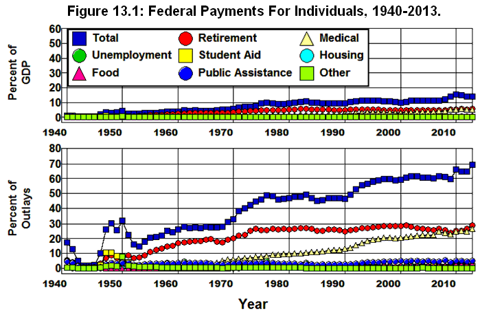
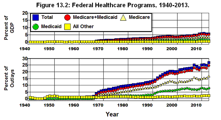
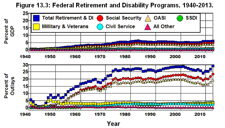
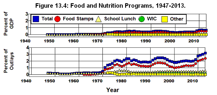
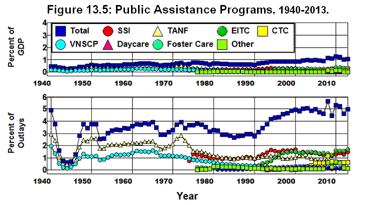
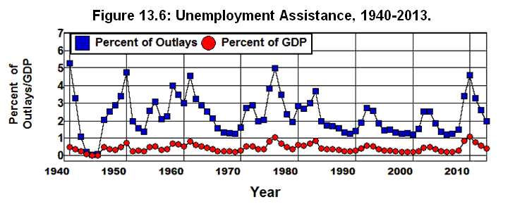
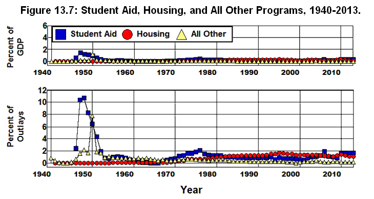
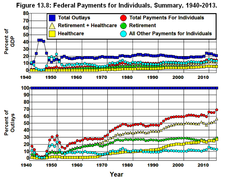
Where Did All The Money Go?
Chapter 14: Welfare, Tax Expenditures, and Redistribution
George H. Blackford © 2010, last updated 5/16/2014
There is no separate account for welfare in the federal budget. As a result, there is no official definition of a welfare program. One way to identify a welfare program is to simply assume that all social-insurance programs are welfare. While some people think this way, people in general see most social-insurance programs as insurance, not welfare, and reject the idea that programs such as Social Security and Medicare are welfare. They view these programs as programs they pay for through payroll taxes, and since they pay for them, they do not consider them to be welfare.
This leads to a problem in defining any social-insurance program as welfare in that all social-insurance programs are paid for through taxes—even those programs that do not have a specific tax associated with them. Since these programs provide insurance throughout an individuals lifetime, not just at a particular point in time, almost everyone pays the taxes that support social-insurance programs at some point in their lives. Even those individuals who do not pay taxes while they are receiving benefits from a social-insurance program either paid the taxes that supported the program from which they are receiving benefits before they began receiving benefits, or they will eventually end up paying those taxes at some point in the future after they no longer in need of the program. Only those who are seriously disabled or otherwise unable to earn an income throughout their entire life find themselves being able to take advantage of social insurance without having to eventually pay the taxes that support social-insurance programs, and, even then, the family members of those individuals generally pay the taxes that support social-insurance programs.
Then there is the argument that those programs in which the recipients benefit by more than they pay in should be considered welfare. This is clearly a fallacious argument. Accepting this argument makes all insurance welfare, private insurance as well as social insurance. The point of insurance is to provide protection against the possibility of catastrophic loss by spreading the risk among the insured. Insurance makes it possible to trade the uncertainty associated with the possibility of a catastrophic loss for the certainty of a smaller loss associated with the cost of the insurance. As a result, those who benefit from any kind of insurance always take out more than they pay in. Those who benefit from fire insurance, for example, when their houses burn down obviously benefit by more than they paid in. That's the way insurance works. It is because insurance makes it possible for people who are faced with a catastrophic loss to benefit by more than they pay in that insurance exists in the first place.
A more common way to draw the distinction between welfare and non-welfare social-insurance is to assume those programs that are means tested—that is, that provide benefits only to the poor that are specifically designed to benefit the less fortunate within our society—are considered to be welfare in spite of the fact that the beneficiaries pay the taxes that support these programs either before or after they receive the benefits from them.
Social Security, Medicare, and unemployment compensation, for example, are not welfare programs under this definition since the benefits of Social Security and Medicare are not means tested and available to those who qualify whether they be rich or poor as are the benefits of unemployment compensation. At the same time, there are a number of social-insurance programs that are means tested, the benefits of which are available only to the indigent or otherwise poor and are specifically designed to transfer income from those who are better off within society to those who are less well off. These are the programs we will examine in this chapter, namely, means-tested programs that provide either cash or non-cash benefits.
Federal Welfare Programs
The federal programs that are means tested in the Office of Management and Budget’s Table 11.3—Outlays for Payments for Individuals are listed in Table 14.1 along with the percentages of GDP and of the federal budget each program represented in 2007.
Table 14.1: Federal Welfare Programs and Expenditures, 2007.
Source: Office of Management and Budget. (11.3 10.1)
* Billions of Dollars
Total expenditures on these programs (Total) are plotted in Figure 14.1 from 1940 through 2013 along with a breakdown of these expenditures on the basis of whether they provide cash (Cash) or non-cash (Non-Cash) assistance.
Source: Office of Management and Budget. (11.3 3.2 10.1)
As is indicated in this figure, total welfare expenditures grew gradually from 1952 through1965 and then began to grow dramatically, increasing from 4.7% of the budget and 0.78% of GDP in 1965 to 16.3% of the budget and 3.1% of GDP in 2007. When we examine the breakdown between cash-payment and non-cash assistance we find that virtually all of the increase in welfare expenditures since 1967 has come about through an increase in non-cash benefits, and that there has been relatively little increase in cash-payment welfare since the early 1960s.
Cash-Payment Welfare
Six of the many means-tested, federal programs listed in Table 14.1 above provide direct cash assistance to low income individuals or families: Supplemental security income program (SSI), Family support payments to States and TANF (TANF), Earned income tax credit (EITC), Payment where child credit exceeds tax liability (CTC, i.e., the Child Tax Credit), Payments to States—Foster Care/Adoption Assist. (Foster Care/Adoption), and Veterans non-service connected pensions (VNSCP). The rest of the programs in Table 14.1 are non-cash assistance programs that provide or pay for specific, in kind benefits such as food, housing, medical care, daycare, etc. Expenditures on each of the cash-payment programs are plotted from 1940 through 2012 in Figure 14.2.
Source: Office of Management and Budget. (11.3 3.2 10.1)
As is shown in this figure, Total expenditures on cash-welfare programs varied between 2.4% and 4% of the budget and between 0.54% and 0.8% of GDP from 1950 through 1990 and amounted to some 4.3% of the budget and 0.83% of GDP in 2007. The increase in cash-welfare programs that took place during the 1990s reflects a fundamental change that took place in our welfare system with the expansion of the Earned income tax credit (EITC) program that was created in 1976, the welfare reform legislation of 1996, and the introduction of the Payment where child credit exceeds tax liability (CTC) program in 1999.
Prior to 1977, the amount of money a cash-welfare welfare recipient earned through employment was subtracted from the amount of assistance he or she received. This created a situation in which there was no incentive for the recipient to accept a job that paid less than his or her cash-welfare benefits since accepting such a job would not increase the recipient's income. This situation was changed with the introduction of the Earned income and Child Tax Credits combined with the replacement of the Aid to Dependent Children program with TANF. Since the benefits of TANF are tied to the willingness of the recipient to find work, and the Earned income and Child Tax Credits are refundable (that is, are paid to the recipient even if the recipient owes no taxes so long as he or she is employed) the effect of these changes is to encourage cash-welfare recipients to seek employment since the benefits of TANF and the Earned income and Child Tax Credit programs are only available to those who are employed or who are participating in an employment training program.
The way in which these welfare reforms have affected the cash-welfare payments by the federal government can be seen in Figure 14.3 where in this figure: Cash Welfare is the total of all cash-welfare payments made by the federal government; Refundable Credits is the amount of money spent by the federal government on the Earned income and Child Tax Credit programs, and Less Refundable Credits is the amount of money spent by the federal government on cash-welfare programs other than refundable tax credits.
Source: Office of Management and Budget. (11.3 3.2 10.1)
As can be seen in this figure, by 2007 almost half (46%) of all federal cash-payment expenditures took the form of refundable tax credits, and even though total cash-welfare expenditures had increased by 15% as a fraction of the budget and 6% as a fraction of GDP since 1976, the amount of federal cash-welfare expenditures that were not tied directly to work through refundable tax credits had fallen by 34% as a fraction of the budget and by 39% as a fraction of GDP by 2007. It is also worth noting that an additional 18% of cash-payment expenditures were made through the Family support payments to States and TANF (TANF) program which has a work requirement associated with it. That means that 64% of all cash-assistance expenditures in 2007 were made through programs designed to encourage work and to assist the working poor.
When we look at the expenditures on the individual cash-assistance programs in 2007 we find that
1.4% of the federal budget and 0.27% of GDP went to the Earned income tax credit (EITC) program to “provide an incentive to work.”
1.2% of the federal budget and 0.23% of GDP went to the Supplemental security income program (SSI) to “help the aged, blind, and disabled who have little or no income by providing cash to meet basic needs for food, clothing, and shelter.”
0.77% of the federal budget and 0.15% of GDP went to the Family support payments to States and TANF (TANF) program to “help move recipients into work and turn welfare into a program of temporary assistance.”
0.59% of the federal budget and 0.11% of GDP went to the Payment where child credit exceeds tax liability (CTC) program to aid lower and middle-income families with children.
0.24% of the federal budget and 0.05% of GDP went to Payments to States—Foster Care/Adoption Assist. (Foster Care) program to aid low income families who provide foster care for and adopt children.
0.12% of the federal budget and 0.02% of GDP went to the Veterans non-service connected pensions (VNSCP) program to aid “wartime Veterans who have limited or no income and who are age 65 or older, or under 65 and are permanently and totally disabled or a patient in a nursing home, or are receiving Social Security disability payments.”
Non-Cash Welfare
As was noted above, all but the six programs plotted in Figure 14.2 are non-cash assistance programs. Here we are talking about Children's health insurance, Medicaid, Indian health, Health resources and services, Substance abuse and mental health services, Student assistance—Department of Education and other, Housing assistance, SNAP (formerly Food stamps) (including Puerto Rico), Child nutrition and special milk programs, Supplemental feeding programs (WIC and CSFP), Low income home energy assistance, Payments to States for daycare assistance, and Other public assistance in Table 14.1.[14.1]
Expenditures on these programs are plotted from 1940 through 2012 in Figure 14.4 where in this figure: Total is the sum of all federal expenditures on non-cash assistance programs listed above; Medicaid is all expenditures on Medicaid; Student Aid is expenditures on Student assistance—Department of Education and other; Housing is the expenditures under the heading Housing assistance; Food is all Food and nutrition assistance expenditures, and Other is the sum of the total expenditures on all of the rest of the non-cash assistance programs listed in Table 14.1 combined.
Source: Office of Management and Budget. (11.3 3.2 10.1)
It is clear from this figure that the total of non-cash assistance programs have increased dramatically since the 1960s, going from 0.7% of the budget and 0.12% of the economy in 1965 to 11.9% of the budget and 2.3% of the economy in 2007. It is also clear from this figure that the reason non-cash assistance programs dominate our welfare system is that the Medicaid program amounted to 6.99% of the budget in 2007 and 1.33% of the economy and, thus, accounted for 43% of all welfare expenditures in 2007 and 58% of all expenditures on non-cash assistance programs. None of the other non-cash assistance programs exceeded 2% of the budget or 0.4% of the economy in 2007. Only 39% of the 11.9% of the federal budget that was devoted to non-cash assistance programs in 2007 went to non-medical welfare programs, and most of the individual non-medical, non-cash programs took up less that 0.25% of the economy.
When we look at the expenditures on the individual programs in 2007, we find that
7.0% of the budget and 1.33% of GDP went to Medicaid,
2.0% of the budget and 0.38% of the GDP went to Food and nutrition assistance programs,
1.2% of the budget and 0.23% of the GDP went to Housing assistance programs,
1.0% of the budget and 0.19% of the GDP went to Student assistance—Department of Education and other programs, and
all of the other non-cash assistance programs combined were 0.75% of the federal budget and 0.14% of the economy.
What about Medicaid? Where did the 7% of the federal budget and 1.3% of gross income earned in 2007 that went to Medicaid go?
The distribution of Medicaid benefits is given in the Census Bureau’s Table 151. Medicaid—Beneficiaries and Payments: 2000 to 2009. Since the data for 2007 is not available in the Census Bureau’s Table 151, the distribution of Medicaid benefits from this table for 2008 are presented in Table 14.2.
Table 14.2 Medicaid Beneficiaries, 2008
Beneficiaries
Total (thousands)
Percent of Total
Expenditures (millions of $)
Percent of Expenditures
Age 65 and over
4,147
7.1
61,131
20.6
Blind/Disabled
8,694
14.8
129,040
43.5
Children
27,111
46.1
51,200
17.2
Adults
12,903
22.0
37,185
12.5
Foster care children
960
1.6
5,936
2.0
Unknown
4,912
8.4
11,825
4.0
BCCA WOMEN
44
0.1
513
0.2
Total
58,771
100.0
296,830
100.0
Source: Census Bureau (151)
Table 14.2 shows that 76% of the known beneficiaries of the Medicaid program in 2008 were either poor Children, Blind/Disabled individuals, or indigent elderly adults Age 65 and over, and over 87% of Medicaid’s expenditures that were classified went to these individuals. Of the 58.8 million Medicaid beneficiaries, only 22% were identified as indigent adults who were not blind/disabled or under age 65, and only 13% of Medicaid’s benefits went to these adults. In other words, less than 1% of the federal budget was spent on Medicaid benefits that went to recipients identified as adults who were not blind/disabled or under age 65.
Entitlements and Welfare
Entitlement's programs are programs that guarantee, by law, specified benefits to anyone who qualifies for the benefits offered by the program. As was noted above, Means-tested programs are designed to provide economic assistance to the indigent and otherwise poor within our society. Since the benefits of means-tested entitlement programs are available only to low income individuals and families they are, by assumption, a form of welfare.
At the same time, an entitlement program may or may not be means-tested and, therefore, may or may not be a form of welfare. Social Security, for example, is an entitlement program that is not a welfare program since its benefits are guaranteed by law to anyone who qualifies for those benefits irrespective of income or wealth, whereas Supplemental Security Income (SSI) is an entitlement program that is a welfare program since its benefits are guaranteed by law only to those who are “aged, blind, [or] disabled who have little or no income.”
The following list of the federal, means-tested entitlement programs can be found in the Section Notes of the Fiscal Year 2013 Historical Tables Budget of the U.S. Government:
• Special milk program
• SNAP (formerly the Food Stamp Program)
• Child Nutrition Programs
• Grants to States for Medicaid
• Children’s Health Insurance Program
• Child Enrollment Contingency Fund
• Payments to States for Child Support Enforcement and Family Support Programs
• Temporary Assistance for Needy Families
• Payment Where Adoption Credit Exceeds Liability for Tax
• Payments to States for Foster Care and Adoption Assistance
• Child Care Entitlement to States
• Payment Where Recovery Rebate Exceeds Liability for Tax
• Payment Where Earned Income Credit Exceeds Liability for Tax
• Payment Where Saver’s Credit Exceeds Liability for Tax
• Health insurance supplement to earned income credit
• Payment Where Child Credit Exceeds Liability for Tax
• Payment Where Credit to Aid First-Time Homebuyers Exceeds Liability for Tax
• Payment Where American Opportunity Credit Exceeds Liability for Tax
• Payment Where Making Work Pay Credit Exceeds Liability for Tax
• Supplemental Security Income Program (SSI)
• Housing Trust Fund
• Veterans’ Pensions benefits
• Refundable Premium Assistance Tax Credit
• Reduced Cost Sharing for Individuals Enrolling in Qualified Health Plans
Figure 14.5 shows the relationship between means-tested entitlement expenditures (Means-Tested Entitlements) and total welfare expenditures (Total Welfare) from 1965 through 2013. While it is clear from this figure that welfare spending is dominated by entitlements in the federal budget—83% of all welfare spending was through entitlements in 2007—the extent to which this is so has varied over the years from a high of 95% federal welfare expenditures in 1964 to a low of 73% in 1986.
Source: Office of Management and Budget. (8.1 10.1 11.3)
Figure 14.5 also shows how the sum of means-tested entitlement programs has grown from 1965 through 2013—from 0.73% of the economy and 4.40% of the federal budget in 1965 to 2.56% of the economy and 13.4% of the federal budget by 2007.
The real story of entitlement programs, however, is told in Figure 14.6 which shows what the growth of means-tested entitlements and welfare expenditures look like with and without Medicaid and refundable tax credits included in the total, and the way in which means-tested entitlements have grown compared to the two largest entitlement programs, Social Security and Medicare.
Source: Office of Management and Budget. (8.1 11.3 10.1)
It is clear from Figure 14.6 that, just as Medicaid dominates the non-cash assistance welfare programs in Figure 14.4, it dominates the means-tested entitlement programs as well. Medicaid was enacted into law in 1965, and by 2007 it accounted for 34% of all government expenditures on means-tested entitlements. Whereas expenditures on non-Medicaid, means-tested entitlements (Means-Tested Entitlements less Medicaid) increased by 77% as a percent of the economy over that 42 year period, because of Medicaid, the sum of all means-tested entitlements (Means-Tested Entitlements) increased by 250%. Means-Tested Entitlements less Medicaid & Tax Credits increased only 22% over this same period.
In other words, almost all of the growth in means-tested entitlements from 1965 through 2007 was in the Medicaid program combined with a significant increase in refundable tax credits and a relatively minor increase in non-Medicaid, non-tax-credit entitlements.
Figure 14.6 also makes it possible to compare the growth of means-tested entitlements from 1965 through 2013 with the sum of the two largest non-means-tested entitlement programs—Social Security and Medicare (Social Security plus Medicare). While means-tested entitlements were growing from 4.4% of the budget and 0.73% of the economy in 1965 to 13.4% of the budget and 2.56% of the economy by 2007, the non-means-tested Social Security and Medicare entitlement programs were growing from 15.5% of the budget and 2.65% of the economy to 37.2% of the budget and 7.09% of the economy. This is, of course, no surprise since we saw in Chapter 13 that Social Security stood at 21.3% of the budget in 2007 and 4.05% of the economy and that Medicare was at 15.9% of the budget and 3.04% of the economy in that year.
Finally, Figure 14.6 shows how the welfare reforms of the 1970s and 1990s have affected entitlements in that Means-Tested Entitlements less Medicaid & Tax Credits shows that non-medical, non-tax-credit entitlement expenditures went from 5.7% of the budget and 1.22% of the economy in 1976 to 4.5% of the budget and 0.88% of the economy in 2007, a decrease of 21% and 28%, respectively.
Tax-Expenditure Entitlements
As we have seen, 4.3% of the federal budget and 0.83% of GDP went to cash-payment welfare programs in 2007, and an additional 11.8% of the budget and 2.3% of GDP went to non-cash welfare programs. These programs are specifically designed to redistribute income from those who are better off within our society to those who are less fortunate. It is important to recognize, however, that welfare programs are not the only way the federal government redistributes income. It also redistributes income through its power to tax.
According to the Joint Committee on Taxation there were over 200 provisions in the federal tax code in 2007 that provided "a special exclusion, exemption, or deduction from gross income or which provide a special credit, a preferential rate of tax, or a deferral of tax liability." Such provisions, which are generally referred to as tax breaks or loopholes, are “designed to encourage certain kinds of behavior by taxpayers or to aid taxpayers in special circumstances . . . [and] may, in effect, be viewed as spending programs channeled through the tax system.” Since the benefits of these "spending programs channeled through the tax system" are guaranteed by law to all who qualify they are, in fact, entitlement programs.
Tax-expenditure entitlement programs play an important role in redistributing income from the general taxpayer to various income groups within our society.
Tax Expenditures and the Redistribution of Income
The Joint Committee estimated that the total of federal tax-expenditures came to more than $1,035 billion in 2007 and that approximately 10% of the benefits of these tax-expenditures went to corporations or other businesses and 90% to individuals. These estimates (which are examined in detail in the Appendix at the end of this chapter) are, in effect, gross estimates in that they only consider how a particular tax expenditure benefits taxpayers directly without considering how eliminating that expenditure will interact with other tax expenditures that affect taxpayers. Nor do they take into consideration how these interactions will affect taxpayers when groups of tax expenditures are eliminated.
Leonard Burman, Eric Toder, and Christopher Geissler at the Tax Policy Center of the Urban Institute and Brookings Institution have examined these interaction effects for the 90% of tax expenditures that benefited individuals and have provided estimates of the way in which tax expenditures affect the after-tax income of various income groups. These estimates for six major categories of tax expenditures (Exclusions, Above-line deductions, Itemized Deductions, Refundable Credits, Non-Refundable Credits, and the special treatment of Capital Gains/Dividends) are summarized in Table 14.3.
Table 14.3: Tax Expenditures as a Percentage of After-Tax Income, 2007.
Program
Quintile
Top 1%
All
1st
2nd
3rd
4th
5th
0.54
2.99
3.79
3.68
4.74
2.9
4.19
0.01
0.06
0.09
0.11
0.08
0.06
0.08
0.02
0.11
0.38
1.09
2.91
3.24
1.97
5.49
5.00
2.20
0.99
0.25
0.00
1.14
0.05
0.28
0.33
0.23
0.06
0.00
0.14
0.00
0.01
0.04
0.12
2.11
5.87
1.26
Total
6.52
8.16
6.76
6.79
11.36
13.53
9.57
Source: Burman, Toder, and Geissler.
This table shows the extent to which after-tax income in each quintile (20%) and the top 1% of the income distribution would be reduced—after adjusting for the interactions between tax expenditures within each category—if each of the six categories of tax expenditures were eliminated as well as if all tax-expenditures were eliminated.
Table 14.3 makes it possible to calculate the average and total benefits received by each income group from each category of tax expenditure in this table as well as the benefits received by each income group from all tax expenditures combined.
Tax Expenditures verses Welfare
In examining Table 14.3 it is apparent that the bulk of the redistribution of income brought about by tax expenditures is from the general taxpayer to the top of the income distribution. The extent to which this is so can be seen in Table 14.4 which shows the average and total benefits received by each income group from all tax expenditures.[14.2]
Table 14.4: Total Tax-Expenditure Benefits by Income Group, 2007.
Income Group
Average After-Tax Income*
x
Benefit / After-Tax Income**
=
Average Benefit
x
Number of Households (Billions)***
=
Total Benefit (billions)
1st Quintile
$17,700
0.0652
$1,154
0.0230
$26.5
2nd Quintile
$38,000
0.0816
$3,101
0.0230
$71.2
3rd Quintile
$55,300
0.0676
$3,738
0.0230
$85.8
4th Quintile
$77,700
0.0679
$5,276
0.0230
$121.1
5th Quintile
$198,300
0.1136
$22,527
0.0230
$517.0
80%-99%
$139,279
0.1028
$14,315
0.0218
$312.1
Top 1%
$1,319,700
0.1353
$178,555
0.0011
$204.9
All
$76,400
0.0957
$7,311
0.1148
$839.1
Sum of Quintiles
=
$821.6
Source: *Congressional Budget Office, **Burman et al., ***Census Bureau.
It is clear from this table that tax expenditures definitely do not have the effect of redistributing income from the general taxpayer to the poor, but rather, have the effect of redistributing income from the general taxpayer to the top of the income distribution. In terms of real money, the $22,527 Average Benefit from all tax expenditures that went to the top 20% of the income distribution in 2007 was almost 20 times greater than the $1,154 Average Benefit that went to the bottom 20% and 6 times greater than the $3,738 Average Benefit that went to the middle 20%.
By the same token, the $178,555 Average Benefit that went to the Top 1% was 155 times greater than the $1,154 Average Benefit that went to the bottom 20%, 48 times greater than the $3,738 Average Benefit that went to the middle 20%, and almost 8 times greater than the $22,527 Average Benefit that went to the top 20% which, of course, includes the Top 1%. When we exclude the Top 1% from the top 20% we find that the Average Benefit of the remaining 19% of the income distribution (80%-99%) was only $14,315 in 2007.[14.3] This is less than 1/12 of the Average Benefit of the Top 1% and is only 3.8 and 12.5 times the Average Benefit of the middle and bottom quintiles, respectively, compared to the 48 and 155 ratios for the Top 1% relative to these quintiles.
More important, however, is the fact that when we compare the absolute magnitude of the Total Benefit received by the various income groups in 2007 we find that the $517.0 billion that went to the top 20% of the income distribution was $73.9 billion greater than the entire $444.7 billion the federal government spent on welfare in that year, and of particular interest is the $204.9 billion of Total Benefit that went to the Top 1%.
The $204.9 billion that went to the Top 1% of the income distribution in 2007—enough to provide an average benefit of $178,555 for each member of the Top 1% in that year—was almost six times the $34.9 billion the federal government spent in 2007 on Food Stamps to provide "nutrition assistance to millions of . . . low income individuals and families" with an average benefit of less than $1,200/year. It was over six times the $32.8 billion spent in 2007 on Supplemental Security Income (SSI) to aid “the aged, blind, and disabled who have little or no income . . . to meet basic needs for food, clothing, and shelter” with its average benefit of $5,244.72/year. And it was almost ten times the $21.1 billion the federal government spent in 2007 on Temporary Assistance to Needy Families to “help move recipients into work and turn welfare into a program of temporary assistance” with its average benefit of less than $10,000/year.
In fact, the $204.9 billion in tax-expenditure Total Benefits that went to the Top 1% of the income distribution in 2007 that provided an Average Benefit of $178,555 for members of the Top 1% of the income distribution in 2007 was more than enough to pay for all of the above welfare programs combined plus the $33.0 billion that went to Housing assistance in 2007, the $27.5 billion that went to Student Aid, the $13.0 billion that went to Child nutrition and special milk programs, the $6.6 billion that went to the Payments to States—Foster Care/Adoption Assist program, the $6.0 billion that went to the Children's health insurance program, the $5.3 billion that went to the Supplemental feeding programs (WIC and CSFP), the $5.1 billion that went to Payments to States for daycare assistance, the $3.4 billion that went to Veterans non-service connected pensions, the $3.2 billion that went to Substance abuse and mental health services, the $3.3 billion that went to Indian health, and the $2.5 billion that went to the Low income home energy assistance program with $5.4 billion left over in change.
In other words, the $204.9 billion the Top 1% of the income distribution saved in taxes as a result of the tax-expenditure entitlement benefits that are built into the tax code—benefits that produced an average government subsidy of $178,555 to the members of the Top 1% of the income distribution in 2007—was enough to fund all of the federal government's welfare programs except Medicaid and that portion of the Refundable Credits program the federal government actually spent on refunds.
What's more, the $312.1 billion in tax-expenditure entitlements that went to the rest of the 19% of the income distribution in the 5th Quintile that provided an Average Benefit of $14,315 to members of the 80%-99% income group was enough to pay for the $190 billion the federal government spent on Medicaid in 2007 plus the $54.5 billion the federal government actually spent on Refundable Credits with $67.5 billion to spare. This $67.5 billion in itself would have been enough to provide an average benefit of $2,945 to each member of richest quintile of the income distribution. This is not only more than twice the $1,153 Average Benefit received by the poorest quintile from all tax expenditures in 2007, it is also more than twice the $1,200 average benefit the federal government paid out in Food Stamps in 2007 to provide "nutrition assistance to millions of . . . low income individuals and families."
It is also instructive to examine the individual categories of tax expenditures summarized in Table 14.3.
Exclusions
Exclusions refers to various forms of income (e.g., scholarships, fellowship grants, welfare benefits, employee fringe benefits, interest on municipal bonds, capital gains transferred at death) that do not have to be reported to the Internal Revenue Service. Exclusions are excluded from gross income.
The average and total benefits received by each income group from Exclusions in 2007 that are implied by Table 14.3 are shown in Table 14.5.
Table 14.5: Benefits from Exclusions by Income Group, 2007.
Income Group
Average After-Tax Income*
x
Benefit / After-Tax Income**
=
Average Benefit
x
Number of Households (Billions)***
=
Total Benefit (billions)
1st Quintile
$17,700
0.0054
$96
0.0230
$2.2
2nd Quintile
$38,000
0.0299
$1,136
0.0230
$26.1
3rd Quintile
$55,300
0.0379
$2,096
0.0230
$48.1
4th Quintile
$77,700
0.0368
$2,859
0.0230
$65.6
5th Quintile
$198,300
0.0474
$9,399
0.0230
$215.7
80%-99%
$139,279
0.0566
$7,880
0.0218
$171.8
Top 1%
$1,319,700
0.0290
$38,271
0.0011
$43.9
All
$76,400
0.0419
$3,201
0.1148
$367.4
Sum of Quintiles
=
$357.7
Source: *Congressional Budget Office, **Burman et al., ***Census Bureau.
This table shows the way in which Exclusions, the largest category of tax expenditures, redistribute income from the general taxpayer to the various income groups within society. Here we find that only $2.2 billion of the $357.7 billion of Total Benefit from Exclusions (less than 1%) went to the poorest quintile (1st Quintile) with an Average Benefit of $96 while some $215.7 billion (60%) went to the richest quintile (5th Quintile) with an Average Benefit of $9,399.
If we break down the richest quintile we find that 20% ($43.9 billion) of the $215.7 billion worth of Total Benefit that went to the top 20% of the income distribution, in fact, went to the Top 1% with an average benefit of $38,271.
The largest beneficiary of the Exclusions tax-expenditure entitlements in terms of Average Benefit is clearly the Top 1% of the income distribution which exceeded the next highest Average Benefit, $7,880 received by the top 80%-99%, by $30,391.
When we compare the bottom 40% (1st Quintile + 2nd Quintile) of the income distribution with top 40% (4th Quintile + 5th Quintile) we find that the bottom 40% received 8% ($28.3 billion) of the $357.7 billion of Total Benefit from Exclusions while the top 40% received more than 79% ($281.4 billion) of these benefits, the difference being $253.1 billion. This $253.1 billion difference was equivalent to 57% of the total of $444.7 billion the federal government spent on welfare in 2007.
Above Line Deductions
Above-Line Deductions are deductions from gross income (e.g., medical insurance premiums for the self employed and standard deductions for the blind and elderly) that taxpayers are allowed to take whether they choose to itemize their deductions or not. Above-Line Deductions are subtracted from gross income to arrive at Adjusted Gross Income.
The average and total benefits received by each income group from Above-Line Deductions in 2007 are shown in Table 14.6.
Table 14.6: Benefits from Above Line Deductions by Income Group, 2007.
Income Group
Average After-Tax Income*
x
Benefit / After-Tax Income**
=
Average Benefit
x
Number of Households (Billions)***
=
Total Benefit (billions)
1st Quintile
$17,700
0.0001
$2
0.0230
$0.0
2nd Quintile
$38,000
0.0006
$23
0.0230
$0.5
3rd Quintile
$55,300
0.0009
$50
0.0230
$1.1
4th Quintile
$77,700
0.0011
$85
0.0230
$2.0
5th Quintile
$198,300
0.0008
$159
0.0230
$3.6
80%-99%
$139,279
0.0009
$125
0.0218
$2.7
Top 1%
$1,319,700
0.0006
$792
0.0011
$0.9
All
$76,400
0.0008
$61
0.1148
$7.0
Sum of Quintiles
=
$7.3
Source: *Congressional Budget Office, **Burman et al., ***Census Bureau.
Above-Line Deductions is the smallest category of tax expenditures in Table 14.3 with only $7.3 billion worth of benefits in 2007. This tax-expenditure entitlement is relatively insignificant, both in terms of the federal budget and in terms of other tax expenditures. Here we find that virtually none of the $7.3 billion of Total Benefit from Above-Line Deductions went to the poorest quintile with an Average Benefit of only $2 while some $3.6 billion (50%) went to the richest quintile with an Average Benefit of $159.
If we break down the richest quintile we find that 25% ($0.9 billion) of the $3.6 billion worth of Total Benefit that went to the top 20%, in fact, went to the Top 1% with an Average Benefit of $792.
When we compare the bottom 40% of the income distribution with the top 40% we find that the bottom 40% received less than 8% ($0.6 billion) of the $7.3 billion worth of Total Benefit from Above-Line Deductions while the top 40% received more than 76% ($5.6 billion) of these benefits, the difference being $5.0 billion. This $5.6 billion was less than 2% of the total amount the federal government spent on welfare in 2007.
Itemized Deductions
Taxpayers can choose between subtracting a fixed Standard Deduction from their adjusted gross income in arriving at their taxable income or of listing separately (itemizing) the individual deductions (e.g., mortgage interest, state and local taxes, medical expenses, charitable contributions, investment interest and other investment and financial expenses) they may be eligible for.
The average and total benefits received by each income group from Itemized Deductions in 2007 are shown in Table 14.7.
Table 14.7: Itemized Deductions by Income Group, 2007.
Income Group
Average After-Tax Income*
x
Benefit / After-Tax Income**
=
Average Benefit
x
Number of Households (Billions)***
=
Total Benefit (billions)
1st Quintile
$17,700
0.0002
$4
0.0230
$0.1
2nd Quintile
$38,000
0.0011
$42
0.0230
$1.0
3rd Quintile
$55,300
0.0038
$210
0.0230
$4.8
4th Quintile
$77,700
0.0109
$847
0.0230
$19.4
5th Quintile
$198,300
0.0291
$5,771
0.0230
$132.4
80%-99%
$139,279
0.0275
$3,824
0.0218
$83.4
Top 1%
$1,319,700
0.0324
$42,758
0.0011
$49.1
All
$76,400
0.0197
$1,505
0.1148
$172.7
Sum of Quintiles
=
$157.7
Source: *Congressional Budget Office, **Burman et al., ***Census Bureau.
Itemized Deductions is the second largest category of tax expenditures. Here we find that only $0.1 billion of the $157.7 billion of Total Benefit from Itemized Deductions (less than 1%) went to the poorest quintile with an Average Benefit of $4 while some $132.4 billion (84%) went to the richest quintile with an Average Benefit of $5,771.
If we break down the richest quintile we find that 37% ($49.1 billion) of the $132.4 billion worth of Total Benefit that went to the top 20%, in fact, went to the Top 1% with an Average Benefit of $42,758.
The largest beneficiary of the Itemized Deductions tax-expenditure entitlement in terms of Average Benefit is clearly the Top 1% of the income distribution which exceeded the next highest Average Benefit, $3,824 received by the 80%-99% income group, by $38,934.
When we compare the bottom 40% of the income distribution with the top 40% we find that the bottom 40% received less than 1% ($1.0 billion) of the $157.7 billion of Total Benefit from Itemized Deductions while the top 40% received 96% ($151.9 billion) of these benefits, the difference being $150.8 billion. This $150.8 billion difference was equivalent to 34% of the $$444.7 billion the federal government spent on welfare in 2007.
Refundable Credits
A tax credit (e.g., the Adoption Credit or Earned Income Tax Credit) is an amount that eligible taxpayers are allowed to subtract from their taxes owed, as determined by their taxable income and the applicable tax rates, in order to determine the amount of taxes they must actually pay.
A Non-Refundable Credits (e.g., the Adoption Credit) is a credit the taxpayer is entitled to only up to the amount of taxes owed. A Non-Refundable Credits cannot reduce the after-credit taxes paid below zero and, thereby, lead to a payment from the government.
A Refundable Credits (e.g., the Earned Income Tax Credit) is a credit for which the taxpayer is entitled to the full amount of the credit whether the credit exceeds the amount of before-credit taxes owed or not. If the amount of a Refundable Credits exceeds the before-credit taxes owed, the taxpayer pays no taxes, and the government must pay (refund) to the taxpayer the difference between the tax credit and the before-credit taxes owed.
The average and total benefits received by each income group from Refundable Credits are shown in Table 14.8.
Table 14.8: Benefits from Refundable Credits by Income Group, 2007.
Income Group
Average After-Tax Income*
x
Benefit / After-Tax Income**
=
Average Benefit
x
Number of Households (Billions)***
=
Total Benefit (billions)
1st Quintile
$17,700
0.0549
$972
0.0230
$22.3
2nd Quintile
$38,000
0.0500
$1,900
0.0230
$43.6
3rd Quintile
$55,300
0.0220
$1,217
0.0230
$27.9
4th Quintile
$77,700
0.0099
$769
0.0230
$17.7
5th Quintile
$198,300
0.0025
$496
0.0230
$11.4
80%-99%
$139,279
0.0037
$522
0.0218
$11.4
Top 1%
$1,319,700
0.0000
$0
0.0011
$0.0
All
$76,400
0.0114
$871
0.1148
$100.0
Sum of Quintiles
=
$122.9
Source: *Congressional Budget Office, **Burman et al., ***Census Bureau.
This table shows the way in which Refundable Credits, the forth largest category of tax expenditures, redistributed income from the general taxpayer to the various income groups within society. Here we find that $22.3 billion of the $122.9 billion of the Total Benefit from Refundable Credits (18%) went to the poorest quintile with an Average Benefit of $972 while only $11.4 billion (9%) of the benefits of this tax expenditure went to the richest quintile with an Average Benefit of $496.
If we break down the richest quintile we find that all of the $11.4 billion worth of Total Benefit that went to the top 20% of the income distribution went to the 80%-99% income group with an Average Benefit of $522. None went to the Top 1%.
The largest beneficiary of the Refundable Credits tax-expenditure entitlement in terms of Average Benefit is the 2nd Quintile of the income distribution with an Average Benefit of $1,900. At the same time, the 3rd Quintile also received a respectable share of the benefits from this tax-expenditure entitlement with an Average Benefit of $1,217, and the 4th Quintile and 80%-99% income group received an Average Benefit equal to 79% ($769) and 51% ($496), respectively, of the $972 Average Benefit received by the poorest quintile.
When we compare the bottom and top 40% of the income distribution we find that the bottom 40% received 54% ($65.9 billion) of the $122.9 billion of Total Benefit from Refundable Credits while the top 40% received only 24% ($29.0 billion) of these benefits, the difference being $36.9 billion. This $36.9 billion was equivalent to 9% of the $$444.7 billion the federal government spent on welfare in 2007.[14.4]
Refundable Credits is the only category of tax expenditure that has the net effect of redistributing income from the general taxpayer to the bottom 40% of the income distribution.
Non-Refundable Credits
The average and total benefits received by each income group from Non-Refundable Credits are shown in Table 14.9.
Table 14.9: Benefits from Non-Refundable Credits by Income Group, 2007.
Income Group
Average After-Tax Income*
x
Benefit / After-Tax Income**
=
Average Benefit
x
Number of Households (Billions)***
=
Total Benefit (billions)
1st Quintile
$17,700
0.0005
$9
0.0230
$0.2
2nd Quintile
$38,000
0.0028
$106
0.0230
$2.4
3rd Quintile
$55,300
0.0033
$182
0.0230
$4.2
4th Quintile
$77,700
0.0023
$179
0.0230
$4.1
5th Quintile
$198,300
0.0006
$119
0.0230
$2.7
80%-99%
$139,279
0.0009
$125
0.0218
$2.7
Top 1%
$1,319,700
0.0000
$0
0.0011
$0.0
All
$76,400
0.0014
$107
0.1148
$12.3
Sum of Quintiles
=
$13.7
Source: *Congressional Budget Office, **Burman et al., ***Census Bureau.
Non-Refundable Credits are the second smallest category of tax expenditures with only $13.7 billion in Total Benefit. This category is rather insignificant compared to the federal budget and the other categories of tax expenditures. Here we find that only $0.2 billion of the $13.7 billion of Total Benefit from Non-Refundable Credits (less than 2%) went to the poorest quintile with an Average Benefit of $9 while $2.7 billion (20%) went to the richest quintile with an Average Benefit of $119.
If we break down the richest quintile we find that all of the $2.7 billion worth of Total Benefit that went to the top 20% of the income distribution went to the 80%-99% income group with an Average Benefit of $125. None went to the Top 1%.
The largest beneficiary of the Non-Refundable Credits tax-expenditure entitlement in terms of Average Benefit is the 3rd Quintile with an Average Benefit of $182, and the 4rt Quintile ran a close second with an Average Benefit of $179. At the same time, the 2nd Quintile and 80%-99% income group received an Average Benefit equal to 58% ($106) and 69% ($125), respectively, of the $182 Average Benefit received by the 3rd Quintile.
When we compare the bottom 40% of the income distribution with the top 40% we find that the bottom 40% received 19% ($2.6 billion) of the $13.7 billion worth of Total Benefit from Non-Refundable Credits while the top 40% received 50% ($6.8 billion) of these benefits, the difference being $4.2 billion. This difference was equivalent to 1% of the $444.7 billion the federal government spent on welfare in 2007.
Capital Gains/Dividends
Most capital gains were taxed at a maximum tax rate of 15% in 2007, rather than at the rates that apply to other forms of taxable income, and qualified dividends were taxed at the same rates as capital gains.
The average and total benefits received by each income group from Capital Gains/Dividends are shown in Table 14.10.
Table 14.10: Benefits from Capital Gains/Dividends by Income Group, 2007.
Income Group
Average After-Tax Income*
x
Benefit / After-Tax Income**
=
Average Benefit
x
Number of Households (Billions)***
=
Total Benefit (billions)
1st Quintile
$17,700
0.0000
$0
0.0230
$0.0
2nd Quintile
$38,000
0.0001
$4
0.0230
$0.1
3rd Quintile
$55,300
0.0004
$22
0.0230
$0.5
4th Quintile
$77,700
0.0012
$93
0.0230
$2.1
5th Quintile
$198,300
0.0211
$4,184
0.0230
$96.0
80%-99%
$139,279
0.0023
$327
0.0218
$7.1
Top 1%
$1,319,700
0.0587
$77,466
0.0011
$88.9
All
$76,400
0.0126
$963
0.1148
$110.5
Sum of Quintiles
=
$98.8
Source: *Congressional Budget Office, **Burman et al., ***Census Bureau.
This table shows the way in which Capital Gains/Dividends, the third largest category of tax expenditures, redistributed income from the general taxpayer to the various income groups within society. Here we find that none of the $98.8 billion of Total Benefit from Capital Gains/Dividends went to the poorest quintile while some $96.0 billion (97%) went to the richest quintile with an Average Benefit of $4,184.
If we break down the richest quintile we find that 93% ($88.9 billion) of the $96.0 billion worth of Total Benefit that went to the top 20% of the income distribution, in fact, went to the Top 1% with an Average Benefit of $77,466. The largest beneficiary of the Capital Gains/Dividends tax-expenditure entitlement in terms of Average Benefit is clearly the Top 1% of the income distribution which exceeded the next highest Average Benefit, $327 received by the 80%-99%, income group by $77,139.
When we compare the bottom 40% of the income distribution with the top 40% we find that the bottom 40% received less than 1% ($0.1 billion) of the $95.5 billion of the Total Benefit from Capital Gains/Dividends went to the bottom 40% while the top 40% received more than 99% ($98.2 billion) of these benefits, the difference being $98.1 billion. This was equivalent to 22% of the $$444.7 billion the federal government spent on welfare in 2007.
Conclusion
It is worth noting that the $77,466 Average Benefit the Top 1% received from the single tax-expenditure entitlement category Capital Gains/Dividends far exceeded the Average Benefit in Table 14.4 from all tax expenditures for any other income group. The next closest was the 80%-99% income group with a total Average Benefit from all tax expenditures of $14,315. It is also fairly safe to say that the $77,466 Average Benefit the Top 1% received from the single tax-expenditure entitlement category Capital Gains/Dividends far exceeded any cash welfare benefit ever received by anyone on welfare.
The special treatment of Capital Gains/Dividends in the tax code is clearly a far more lucrative welfare program for the wealthy than any welfare program available to the poor.
Appendix on Gross Tax Expenditures
In its 2007 report, Estimates of Federal Tax Expenditures for Fiscal Years 2007-2011, the Joint Committee on Taxation provided estimates of all federal tax-expenditure programs that were expected to reduce federal tax revenue by $50 million or more over the course of five years. Of the 172 programs the committee so identified, the 31 largest are itemized in Table 14.11 below along with the total expenditure (i.e., expected revenue loss) associated with each program in 2007 and the percentages of the budget and of GDP that the program's expenditure represented. These are gross tax expenditures in that they estimate by how much government revenue was reduced as a result of each program without considering the way in which tax-expenditure programs interact were a given program or group of programs to be eliminated.
The 31 programs itemized in Table 14.11 include all of the programs identified by the Joint Committee on Taxation that were expected to cost the federal government $5 billion (i.e., 0.18% of the budget or 0.04% of GDP) or more in 2007 where 2007 has been chosen as the year of comparison because that was before the current economic crisis began to take its toll and distort the federal budget. These were the largest tax-expenditure entitlement programs in the federal budget in 2007, and they accounted for $912 billion of the $1,035 billion worth of tax expenditures identified by the committee.
Table 14.11: Major Tax-Expenditure Programs, 2007.
Program
Billions of Dollars
Percent of Budget
Percent of GDP
General Science, Space, and Technology
6.4
0.23
0.05
5.1
0.19
0.04
Other General Science, Space, and Technology
1.3
0.05
0.01
International affairs
18.9
0.69
0.14
Deferral of active income of controlled foreign corporations
5.8
0.21
0.04
6.4
0.23
0.05
Other International affairs
6.7
0.25
0.05
General Purpose Fiscal Assistance
61.7
2.26
0.45
Exclusion of interest on public purpose State and local government bonds
27.8
1.02
0.20
33.9
1.24
0.24
Education and training
18.7
0.69
0.13
Deduction for charitable contributions to educational institutions
6.6
0.24
0.05
Other Education and training
12.1
0.44
0.09
Employment
42.3
1.55
0.31
30.0
1.10
0.22
6.6
0.24
0.05
Other Employment
5.7
0.21
0.04
Social Services
83.1
3.05
0.60
45.0
1.65
0.32
Deduction for charitable contributions other than for education and health
33.8
1.24
0.24
Other Social Services
4.3
0.16
0.03
Housing
131.1
4.80
0.95
Deductibility for mortgage interest on owner-occupied residences
73.7
2.70
0.53
16.8
0.62
0.12
28.5
1.04
0.21
5.1
0.19
0.04
Other Housing
7.0
0.26
0.05
Income Security
215.9
7.91
1.56
Net exclusion of pension contributions and earnings: Employer plans
108.6
3.98
0.78
15.5
0.57
0.11
Plans covering partners and sole proprietors (sometimes referred to as "Keogh plans")
8.8
0.32
0.06
Exclusion of untaxed social security and railroad retirement benefits
22.4
0.82
0.16
44.7
1.64
0.32
Other Income Security
15.9
0.58
0.11
Healthcare
176.9
6.48
1.28
105.7
3.87
0.76
8.4
0.31
0.06
Exclusion of workers' compensation benefits (medical benefits)
7.5
0.27
0.05
40.9
1.50
0.30
Other Healthcare
14.4
0.53
0.10
Commerce
250.9
9.19
1.81
Exclusion of investment income on life insurance and annuity contracts
28.6
1.05
0.21
Reduced rates of tax on dividends and long-term capital gains
127.1
4.66
0.92
51.9
1.90
0.37
5.5
0.20
0.04
5.6
0.21
0.04
Deduction for income attributable to domestic production activities
5.2
0.19
0.04
Other Commerce
27.0
0.99
0.19
Other Tax Expenditure Programs
29.1
1.07
0.21
Total of Major Tax Expenditure Programs
1,035.0
37.93
7.47
Source: Joint Committee on Taxes. (1)
Science, International, and Fiscal Assistance
The purposes of tax-expenditure entitlements that fall under the headings of General Science, Space, and Technology, International affairs and General Purpose Fiscal Assistance in Table 14.11 are relatively straightforward and are only tangentially related to the concept of income redistribution. In any event, tax-expenditures on these programs amounted to some $86.0 billion in 2007, were equivalent to 3.2% of the federal budget, and accounted for some 8.3% of the tax expenditures identified by the Joint Committee in 2007.
The tax-expenditure entitlements that are most closely associated with our welfare programs are to be found under the headings Education and training, Employment, Social Services, Housing, Income Security, Healthcare, and Commerce.
Education and Training
The programs designed to promote Education and Training are relatively insignificant. The only program that exceeded $5 billion in expected forgone revenue in 2007 was the $6.6 billion that went to Deduction for charitable contributions to educational institutions. This amounted to only 0.24% of the budget and 0.05% of GDP in that year, and, in total, tax expenditures Education and Training amounted to only $18.7 billion and 0.69% of the budget and 0.13% of GDP.
These programs, undoubtedly, aid some in the lower income groups.
Employment
Employment fared somewhat better in the federal tax-expenditure budget with two programs that exceed $5 billion in 2007:
$30 billion that went to Exclusion of benefits provided under cafeteria plans.
$6.6 billion that went to Exclusion of miscellaneous fringe benefits.
This $36.6 billion of expected forgone revenue provided a subsidy to those who receive a portion of their income in the form of in-kind fringe benefits. These programs were equivalent to 1.34% of the budget and 0.27% of GDP in 2007, and the total for this category ($42.3 billion) amounted to 1.55% of the budget and 0.31% of GDP.
Social Services
Social Services also had two programs that exceeded $5 billion in the tax-expenditure budget:
$45.0 billion for the Tax credit for children under age 17.
$33.8 billion for Deduction for charitable contributions other than for education and health.
Here we find the Tax credit for children under age 17 which amounted to 1.24% of the federal budget and 0.24% of GDP in 2007, and Deduction for charitable contributions other than for education and health which amounted to 1.24% of the federal budget and 0.24% of GDP in 2007. The sum of these two items under Social Services came to 2.89% of the budget and 0.57% of GDP in 2007, and the total for this category ($83.1 billion) came to 3.05% of the budget and 0.60% of GDP.
Housing
Four programs exceeded $5 billion under the heading Housing in Table 14.11:
$73.7 billion for Deductibility for mortgage interest on owner-occupied residences,
$16.8 billion for Deduction for property taxes on owner-occupied residences,
$28.5 billion for Exclusion of capital gains on sale of principal residence.
$5.1 billion for Tax credit for low-incoming (sic) housing.
The sum of these four subsidies ($124.1 billion) amounted to 4.55% of the federal budget and 0.89% of GDP in 2007, and the total for this category ($131.1) came to 4.80% of the budget and 0.95% of GDP.
Of these four items, only the $5.1 billion Tax credit for low-incoming housing expenditure (4.1% of the total) is designed to benefit the poor. The rest of these programs are designed to benefit middle and upper income groups who can afford to own their own home.
In comparing these tax-expenditures to the federal Housing assistance welfare programs we find that the gross tax-expenditure subsidies in Housing that went to middle and upper income groups far exceeded the welfare Housing assistance that went to indigent individuals and the working poor. In fact they were more than three and a half times the $32.0 billion in welfare Housing assistance expenditures that went to indigent individuals and the working poor in 2007.
Healthcare
There are also four programs that exceeded $5 billion under the heading Healthcare in Table 14.11:
$105.7 billion for Exclusion of employer contributions for health care, health insurance. premiums, and long-term care insurance premiums.
$8.4 billion for Deduction for medical expenses and long-term care expenses.
$7.5 billion for Exclusion of workers' compensation benefits (medical benefits).
$40.9 billion for Exclusion of Medicare benefits in excess of cost.
These subsidies amounted to $162.5 billion in 2007 and were equivalent to 5.95% of the budget and 1.17% of GDP, and the total in this category ($176.9 billion) came to 6.48% of the budget and 1.28% of GDP.
These gross benefits from the programs accrued mostly to the middle and upper income groups, and while this $176.9 billion federal entitlement subsidy in Healthcare is somewhat less, it is of the same order of magnitude as the federal healthcare subsidy provided by the federal Medicaid program which amounted to $190.6 billion and was equal to 6.99% of the budget and 1.37% of GDP in 2007.
Income Security
Next we come to Income Security which contains five programs that exceed $5 billion in forgone revenue by the federal government:
$108.6 billion for Net exclusion of pension contributions and earnings: Employer plans.
$15.5 billion for Individual retirement plans.
$8.8 billion for Plans covering partners and sole proprietors (sometimes referred to as "Keogh plans").
$5.5 billion for Exclusion of untaxed social security and railroad retirement benefits.
$44.7 billion for Earned income credit (EIC).
Here we find the Earned income tax credit (Earned income credit (EIC) which amounted to some $44.7 billion in 2007, 1.64% of the budget, and 0.32% of GDP. This program is specifically designed to benefit lower income groups.
The fourth program under the Income Security heading in Table 14.11, Exclusion of untaxed social security and railroad retirement benefits, is relatively insignificant at only $5.5 billion, but the other three programs that fall under the Income Security heading are significant, especially when they are combined. Net exclusion of pension contributions and earnings: Employer plans, Individual retirement plans, and Plans covering partners and sole proprietors (sometimes referred to as "Keogh plans") all subsidize various forms of private pension plans. The cost of these three subsidies summed to $132.9 billion in 2007, and they were equivalent to 4.87% of the federal budget and 0.95% of the GDP in that year.
When we compare the $132.9 billion paid out through these three tax expenditure entitlement programs—which mostly benefited middle and upper-income individuals—to the cash welfare payments from the Supplemental Security Income (SSI) program that went to “the aged, blind, and disabled who have little or no income . . . to meet basic needs for food, clothing, and shelter” in 2007 we find that these three programs provided benefits that were four times the $32.8 billion in benefits paid out by SSI. In fact, these three tax-expenditure entitlement subsidies provided a benefit to middle and upper income groups that was greater than the entire $123.5 billion federal cash-payment welfare budget in 2007.
Commerce
Finally, we get to the last major heading in Table 14.11 that has yet to be examined: Commerce. Six tax-expenditure programs exceeding $5 billion in tax expenditures fell under this heading in 2007:
$127.1 billion for Reduced rates of tax on dividends and long-term capital gains.
$51.9 billion for Exclusion of capital gains at death.
$28.6 billion for Exclusion of investment income on life insurance and annuity contracts.
$5.6 billion for Deduction for income attributable to domestic production activities.
$5.5 billion for Carryover basis of capital gains on gifts.
$5.1 billion for Deferral of gain on non-dealer installment sales.
These six programs amounted to $223.8 billion in 2007 and would appear to have little purpose in the tax code other than to benefit middle and upper-income groups within our society. They were equivalent to 8.20% of the budget and 1.61% of GDP in 2007, and the total in this category ($250.9 billion) came to 9.19% of the budget and 1.81% of GDP.
This $250.9 billion tax-expenditure entitlement subsidy to the middle and upper-income groups within our society amounted to $47.6 billion more that the $203.3 billion the federal government paid out in medical benefits to the indigent and working poor in 2007 and was actually $11.1 billion greater than the entire $239.8 billion the federal government spent on all federal non-medical welfare programs in that year.
Appendix on Welfare in 2013
Table 13.2 gives the welfare expenditures in the Office of Management and Budget’s Table 11.3—Outlays for Payments for Individuals for each program in 2012 along with the percent of GDP and of the federal budget that each program represented in that year.
Table 14.12: Federal Welfare Programs and Expenditures, 2013.
Source: Office of Management and Budget. (11.3 10.1)
Endnotes
[14.1] The extent to which Other public assistance programs should be included in cash-payment or non-cash-welfare programs is not clear. This item is arbitrarily included in non-cash-payment programs for present purposes, but it is important to realize that these programs represented only 0.01% of the budget in 2007 and, thus, represent little more than rounding error in the numbers that follow or those that have been discussed above.
[14.2] The Average Benefit in this table is obtained by multiplying the Tax Expenditures as a Percentage of After-Tax Income for Total in Table 14.3 (i.e., the Benefit / After-Tax Income column in Table 14.4 is obtained from the line for Total in Table 14.3) by the Average After-Tax Income that is provided by the Congressional Budget Office for each income group. The Total Benefit in Table 14.4 is calculated by multiplying the number of households in each group as provided by the Census Bureau by the Average Benefit of each income group.
[14.3] The 80%-99% income group is not contained in Table 14.3, but the Total Benefit received by this income group is easily calculated by subtracting the Total Benefit received by the Top 1% from those received by the 5th Quintile. The Number of Households in this group is give by difference between the number of households in the 5th Quintile and Top 1%, and the Average Benefit is given by the ratio of Total Benefit and the Number of Households in this group. Since the average income of the 5th Quintile (Y5) is equal to the Total Income in this quintile divided by the Number of households in each quintile (N), the average income of this quintile is given by:
(1) Y5 = [Y19x(19/20)N + Y1x(N/20)] / N,
where Y19 and Y1 are the average incomes of the 80%-99% and Top 1% income groups, respectively. Thus, the Average Income of the 80%-99% income group is given by:
(2) Y19 = (Y5 - Y1/20) x ( 20/19).
It should also be noted that the Excel spreadsheet by which all of the calculations in this note have been made can be downloaded by clicking on this link.
[14.4] It should be noted that there is a bit of double counting here. The $122.9 billion of the Total Benefit from the Refundable Credits includes the refunded portion of this tax expenditure which amounted to over $54.5 billion in 2007. The refunded portion of this tax expenditure was an actual expenditure in the federal budget in 2007 and is included in the total of $444.7 billion the federal government spent on welfare in that year.
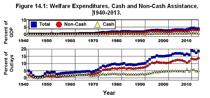
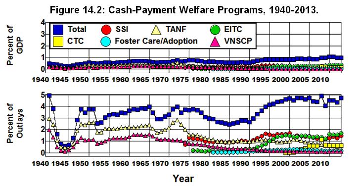
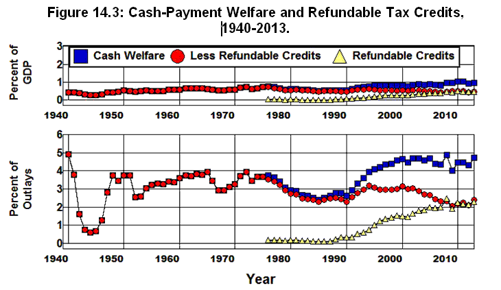
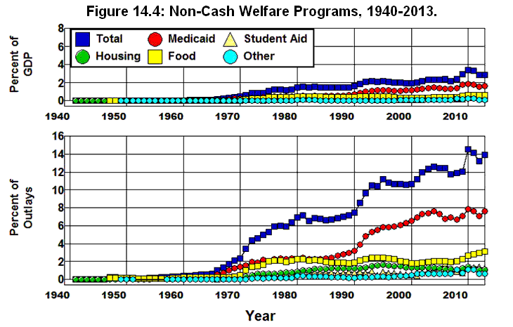
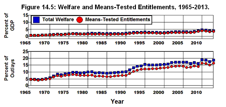
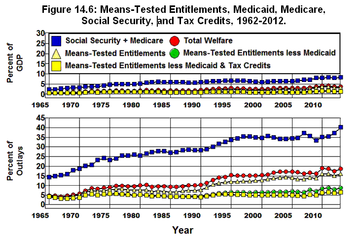
Where Did All The Money Go?
Chapter 15: Federal Versus Non-Federal Debt
George H. Blackford © 2012, last updated 5/16/2014
This chapter examines the fundamental difference between federal debt and non-federal debt and the lessons that should have been learned from the 1930s with regard to the importance of this difference as it relates to economic policy and the stability of the economic system.
Managing the Federal Budget
There is a fundamental difference between federal debt and non-federal debt that arises from the fact that the federal government has the legal right to print money. Since the federal government can print money there is no reason to believe it will ever be unable to service its debt since it can always print the money it needs if it has to. Non-federal debtors cannot print money. They must service their debts out of income or through the sale of assets and, as a result, are always at risk of being unable to meet their financial obligations.
The fact that the federal government has the power to print money does not mean we do not have to worry about federal debt or that “deficits don’t matter” as was the mantra of the Bush II administration. It matters a lot just how those deficits are created and how they are financed, but the fact that the federal government has the power to print money means that the federal debt problem is a much easier problem to deal with than the non-federal debt problem. It also means that the federal government has the power to mitigate the overall debt problem we face through the judicious management of its budget in a way that non-federal debtors do not.
When the federal government borrows and uses the proceeds to finance an increase in expenditures for goods and services in the face of an economic downturn it increases spending in the economy directly and thereby directly increases the demand for goods and services.
The same is true when the government borrows in this situation to increase transfer payments (such as increased payments for agricultural subsidies, unemployment compensation, or aid to municipalities) or to finance tax cuts that created the need to borrow in the first place, though here the effect on the demands for goods and services is less certain in that these effects are indirect. They can have an effect on the demands for goods and services only to the extent that those who received the transfer payments or tax cuts increase their spending as a result. There is, of course, no guarantee this will occur.
Deficits that occur during an economic downturn that help to maintain or increase expenditures on education, scientific research, public health systems, police and fire protection, bridges, highways, and other forms of public transportation all have the direct effect of stimulating the economy. Even expenditures that arise from increases in the kinds of transfer payments embodied in food stamps, unemployment compensation, school lunch programs, Medicaid, and other kinds of social welfare programs that tend to increase during an economic downturn help to stimulate the economy since most of these transfers go to people who live hand to mouth, and, therefore, are more or less forced to spend.
In addition, most, if not all of these kinds of expenditures, whether direct expenditures or social welfare transfers, have the added benefit of making it possible to improve productivity in the future by improving our public infrastructure and warding off the malnutrition and other health problems that are the inevitable consequence of people becoming destitute in the wake of an economic downturn. Thus, running a deficit to finance these kinds of expenditures and transfer payments during an economic downturn adds stability to the system and has the potential to help the economy grow and, thereby, to reduce the burden of servicing the debt that deficits create.
By the same token, deficits that occur during prosperous times or that are created in the midst of an economic downturn by giving tax cuts and increasing transfer payments to the ultra wealthy who, in turn, use the proceeds to buy the bonds needed to finance the deficits created by the transfers and tax cuts in the first place do not stimulate the economy and do not have the added benefit of having the potential to improve productivity in the future. They simply increase the transfer burden from debtors (i.e., taxpayers) to creditors as they distort the allocation of resources within the system with a dead loss to the society as a whole. In addition, this kind of fiscal irresponsibility on the part of the government has the potential to create chaos within the economic system.
Even though there is no default risk to federal debt, when federal debt grows faster than the GDP it increases the burden of transfers from debtors to creditors which can lead to serious problems, especially if the debt is foreign owned. In addition, there is a huge risk of inflation as the federal debt grows if it reaches the point where the government cannot raise the money to service its debt through taxes or borrowing and is forced to print money. The resulting inflation can have the effect of increasing interest rates and, thereby, making the transfer problem worse as it weakens our position in international markets. If severe enough, hyperinflation can lead to a total collapse of the monetary system as creditors refuse to enter into contracts of any sort that are written in terms of the domestic currency.
Thus, the ability of the federal government to print money is not a blank check that allows the federal government to do whatever it chooses. It only gives the federal government a degree of flexibility in managing its affairs that no other entity within the economic system has, but the federal budget must be managed responsibly if catastrophe is to be avoided. This does not mean that the budget should always be balanced or that federal debt should be paid off as quickly as possible. As we will see, attempting to do so can have disastrous consequences.
What it does mean, however, is that during an economic downturn the deficit and debt must be increased in such a way as to maximize the economic stimulus while, at the same time, alleviating human misery and building up our public infrastructure as much as possible in order to minimize the economic decline and increase our ability to produce in the future. It also means eliminating unproductive or wasteful programs and expenditures during prosperous times and increasing taxes to pay for the government programs and expenditures that are essential to our economic and social wellbeing.
Not managing the budget in this way and, in particular, not increasing taxes to pay for the government programs and expenditures that are essential to our economic and social wellbeing while giving tax cuts to those who have no need to spend the proceeds during an economic downturn is courting disaster. (Stiglitz Klein Johnson Crotty Bhagwati Philips Galbraith Morris Reinhart Kindleberger Smith Eichengreen Rodrik Krugman)
Non-Federal Debt
In spite of the fact that 80% of our total debt is non-federal debt, there has been an extraordinary amount of concern since 2008 over the growing national debt. This concern is dangerously misplaced. It is the $47 trillion of non-federal debt that existed at the end of 2013 that we should be most concerned about, not the $12 trillion federal debt. The most serious problem we face today is the fact that the non-federal debt stood at 278% of GDP in 2013. As was noted in Chapter 3, a ratio of this magnitude places a huge transfer burden on the financial system, a burden that places the entire economic system at risk.
The fundamental problem faced by non-federal debtors is that they must service their debts out of income. When they cannot service their debts out of income they must refinance their debts when they come due, and, failing that, they are forced to sell assets. If they lack the assets to sell, their only option is to default.
As was explained in Chapter 5, and elaborated on in Chapter 6 and Chapter 10, the forced selling of assets and defaults on non-federal debt leads to falling asset prices that threaten the solvency of those financial institutions that hold similar kinds of assets, not just the creditors of those who sell assets or default on their debts. Since all of the major financial institutions hold similar kinds of assets, a non-federal debt ratio as high as 278% of GDP poses a threat to the entire financial system in that it imposes such a transfer burden on debtors that even a minor shock to the system, such as an increase in interest rates or a slowdown in the rate of growth of GDP, has the potential to initiate a wave of distress selling and defaults that puts the entire financial system at risk. This is, of course, what was in the process of happening in 2007 through the summer of 2009.
The increase in interest rates from 2005 through 2007 led to a fall in housing prices and increasing defaults in the mortgage market which, in turn, led to the downturn in economic activity we experienced from the fall of 2007 through the summer or 2009. This left financial institutions in a precarious situation as they struggled to get as many risky assets off their books as possible for fear of being forced into insolvency should the economic situation get worse. At the same time, debtors found it more difficult to refinance their debts, and many financial institutions were forced to refinance existing loans in order to avoid having to take a loss on those loans. As a result, the financial intermediation process broke down as debtors found it more difficult to meet their financial obligations; financial institutions began to fail, and those that survived refused to make new loans and resisted refinancing existing loans. It took the heroic actions of the Federal Reserve and tremulous actions of the federal government examined in Chapter 10 to keep the system form collapsing.
It should be obvious that if the federal government had attempted to balance its budget by cutting its expenditures in this situation the result would have been an even further fall in the economy. This would have decreased the amount of spending which would have forced an even greater number of non-federal debtors to liquidate assets or default on their financial obligations in a situation in which the entire financial system was on the verge of collapse.
It should also be obvious that it is going to be virtually impossible for financial institutions to intermediate between borrowers and lenders in such a way as to allow the economy to recover from this crisis in a reasonable amount of time without further government stimulus since the only way financial intermediation can do this is by increasing debt, and it is virtually impossible for financial intermediation to increase debt with a non-federal debt ratio of 278% in the absence of massive investment opportunities, real or imagined, to justify this increase.
Given the experiences we have had with imaginary investment opportunities over the past thirty years and the disastrous consequences that have followed, it is unlikely we will be able to rely on another stock market or real estate bubble to provide yet another temporary solution to this problem. And since the real investment opportunities needed to accomplish this are wanting, we are not likely to be able to get out of the hole we have dug ourselves into through yet another massive increase in debt.
At the same time, there is no reason to think we can solve this problem by purging the system of debt by balancing the federal budget and forcing debtors to default through conservative monetary and fiscal policy. That certainly didn’t work in the 1930s.
Purging Debt in the 1930s
Figure 15.1 shows the relationship between GDP and total, non-federal, and federal debt from 1929 through 1941. It also shows what happened when the system was allowed to purge itself of debt from 1929 through 1933 by forcing debtors to liquidate their assets or default.
Source: Historical Statistics of the U.S. (Cj870), Bureau of Economic Analysis (1.1.5).
As non-federal debt fell from $175 billion in 1929 to $144 billion in 1933, GDP fell from $105 billion to $57 billion. Thus, in the process of purging $31 billion worth of non-federal debt from the system GDP fell by $47 billion. The end result was an 18% fall in non-federal debt accompanied by an 45% fall in GDP as the ratio of non-federal debt to GDP went from 168% of GDP to 252% of GDP. In the meantime, over 10,000 banks failed along with 129,000 other businesses; the unemployment rate soared to 25% of the labor force, and 12 million people found themselves unemployed by the time this purging of debt came to an end. This was the legacy of Andrew Melon's infamous advice to Herbert Hoover:
. . . liquidate labor, liquidate stocks, liquidate farmers, liquidate real estate… it will purge the rottenness out of the system. High costs of living and high living will come down. People will work harder, live a more moral life. Values will be adjusted, and enterprising people will pick up from less competent people. (Hoover)
The purging of debt from 1929 through 1933 led us into the depths of the Great Depression, and it is instructive to examine just how we got there.
Monetary Policy, 1929-1933
Figure 15.2 shows the gross domestic product deflator along with the money supply, High-Powered Money, and member bank reserves from 1929 through 1941.[15.1]
Source: Bureau of Economic Analysis, (1.1.6A), Economic Report of the President 1960 (D40 D42).
As is shown in this figure, the demand for currency outside of banks was unchanged in 1929 and 1930 as currency in circulation remained at $3.6 billion in both of those years. It then increased by $900 billion in 1931 as the banking crisis that began in October of 1930 took hold and increased by an additional $200 million in 1932. By 1933 currency in circulation stood at $4.8 billion and had increased by a total of $1.2 billion since 1930.
This 33% increase in demand for currency outside of banks was met by an increase in High-Powered Money that followed a similar pattern as the increase in the demand for currency, but with a lag: High-Powered Money remained unchanged at $6.0 billion in 1929 and 1930, increased by $844 million in 1931, actually fell by $9 million in the midst of the crisis in 1931 as member-bank reserves fell by $200 million, and then increased by $329 million as the total increased to $7.1 billion in 1933.
This lag in the creation of High-Powered Money on the part of the Federal Reserve, combined with the overall timidity of its response to the crisis, allowed member-bank reserves to fall by $265 million from 1930 through 1932 as banks struggled to maintain their solvency in the face of falling asset prices brought on by the stock market crash and the economic downturn that followed. As a result, the money supply began to fall in 1930 as banks tried to improve their financial situation by refusing to make new loans or to renew existing loans in an attempt to hang on to their reserves. In the process, currency plus all deposits fell by 22% from 1929 through 1933 (from $54.7 billion to $42.6 billion) while currency plus demand deposits fell by 25% (from $26.4 billion to $19.8 billion).
In turn, the process by which this contraction of the money supply took place—banks refusing to make new loans or to renew existing loans—had a devastating effect on prices as business were forced to mark down their inventories and sell them off at a loss. It also had a devastating effect on wages as employers found it impossible to maintain the level of wages they had previously been able to pay as the prices at which they were able to sell the output they produced fell.
The deflation that resulted from 1929 through 1933 as the Federal Reserve sat back and allowed the system to purge its debt is clearly shown in Figure 15.2 by the 26% fall in the GDP deflator from 119 in 1929 to 88 in 1933.
Fiscal Policy, 1929-1933
Figure 15.3 shows the total outlays, receipts, and surpluses of the federal government from 1929 through 1941 along with the rate of unemployment and the output of goods and services as given by real GDP measured in 1937 prices.
Source: Bureau of Economic Analysis, (3.2 1.1.6A), Economic Report of the President, 1967 (B20).
As is shown in this figure, federal government expenditures gradually increased from 2.8% of GDP in 1929 to 6.5% in 1933 as actual expenditures increased from $2.9 billion to $3.7 billion and tax receipts fell from $3.7 billion to $2.6 billion. In the process the budget went from a $800 million surplus to a $1.1 billion deficit.
In the meantime, real GDP measured in 1937 prices fell from $88.2 billion to $65.0 billion, a 26.3% decrease in the output of goods and services produced. When this fall in output was combined with 25% fall in prices shown in Figure 15.2 it brought about the 46% fall in GDP shown in Figure 15.1. Thus, while non-federal debt decreased by $31.2 billion during this period, this decrease was partially offset by a $7.8 billion increase in federal debt as tax revenues fell and emergency spending increased. At the same time, GDP fell from $104 billion in 1929 to $56 billion in 1933 as the total debt ratio exploded from 183% to 295% of GDP and, as was noted above, the non-federal debt ratio increased from 168% to 252% of GDP.
In the end, a net $23 billion of debt was purged from the system by forcing debtors to liquidate their assets or to default on their debts, a reduction equal to 22% of the total in 1929. In the process of purging this debt, the total debt to GDP ratio—and along with it, the burden of servicing the remaining debt—went through the roof as this ratio increased by 111 percentage points to 283% of GDP and the non-federal debt ratio increase by the 84 percentage points to 252% of GDP as gross income (i.e., nominal GDP) fell by 45% and output (i.e., real GDP) by 26%. And it is worth emphasizing again that along the way over 10,000 banks failed along with 129,000 other businesses; the unemployment rate soared to 25% of the labor force, and 12 million people found themselves unemployed by the time this purging of debt came to an end.
Deleveraging, 1933-1936
It wasn’t until after the Federal Reserve allowed High-Powered Money to increase dramatically following 1933 (Figure 15.2) in a way that allowed banks to increase their excess reserves dramatically—from virtually zero ($60 million) in 1931 to $770 million in 1933 to $1.8 billion in 1934 and to $3.0 billion in1935—that the purging of debt came to an end. And it wasn’t until after government expenditures had increased to 10.7% of GDP ($6.6 billion) and the government’s budget had gone from a surplus equal to 0.7% of GDP in 1929 to a deficit (negative surplus) of 5.9% of GDP ($3.6 billion) in 1934 (Figure 15.3) that debt stopped falling and the rate of unemployment began to fall as GDP began to increase (Figure 15.1).
In other words, the debt problem that was created in the 1920s and was allowed to cripple the economy from 1929 through 1933 was not resolved by forcing debt to be purged from the system through conservative monetary and fiscal policies. It was resolved through the active participation of the Federal Reserve in providing the excess reserves needed by the banking system to end the implosion of the financial system that took place from 1929 through 1933, and through the active participation of the federal government to stimulate the economy through an increase in government expenditures that increased the demand for goods and services and made it possible for the economic system to grow.
Even then it took the 1933 bank holiday in which all the banks were forced to close and then reopened with a deposit guarantee on the part of the federal government before the carnage caused by the downward spiral of debt, GDP, and employment was brought to an end.
It is also worth noting that the deleveraging in the economy that took place as the total debt ratio went from 295% of GDP in 1933 to 163% by 1941 took place through an increase in GDP, not through a decrease in debt. Total debt increased from $168 billion in 1933 to $211 billion in 1941 while non-federal debt increased from $144 billion to $155. At the same time GDP went from $57 billion to $129 billion. (Figure 15.1) Clearly, it was the increase in GDP that was facilitated by the increase in government expenditures and expansionary monetary policy that led to the decrease in the debt ratio following 1933, not a fall in debt.
The 1936-1938 Debacle
Yet another important lesson to be learned from the 1930s, that has particular relevance today, is the results of the change in government policy following 1936 as federal government attempted to balance its budget by cutting its expenditures and the Federal Reserve increased reserve requirements in an attempt to eliminate the excess reserves in the banking system.
As the federal expenditures and excess reserves began to fall from 1936 through 1938 (Figure 15.2 and Figure 15.3) the increase in output ended and GDP began to fall again as the rate of unemployment and the debt ratios began to rise. In other words, when the federal government cut its expenditures in 1936 through 1938 and the Federal Reserve tried to eliminate the excess reserves in the banking system during this period, the economic recovery ended and the economy slipped back into a recession. The economic system did not recover from this shock until the federal government and Federal Reserve reversed their policies and government expenditures and excess reserves began to increase again after 1938.
The government’s attempt to return to conservative monetary and fiscal policy in 1936 managed to reduce the excess reserves in the banking system by 68% in 1937 and to nearly balance the federal budget in 1938, but at the cost of a jump in unemployment from 15.6% of the labor force in 1937 to 18.1% in 1938 as the output of goods and services fell by 3.5%, and the federal debt to GDP ratio went from 42.7 in 1937 to 46.2 in 1939. It is exceedingly difficult to explain just how the benefits gained, whatever them may have been, from this exercise in conservative monetary and fiscal policy justified these costs.
Lessons from the 1930s
There are at least three fundamental lessons that should have been learned from our experiences during the Great Depression.
Conservative Policies Do Not Work
The first lesson that should have been learned from the 1930s is that implementing a conservative monetary and fiscal policies that forces non-federal debt to be purged from the system by forcing debtors to liquidate their assets and default on their financial obligations in the face of an economic downturn is not a good idea. Such policies drove the system into a downward spiral from 1929 through 1933 that didn’t come to an end until after those policies came to an end.
The importance of this lesson is reinforced by the fact that when these self-defeating policies were resumed following 1936 the economic recovery that their abandonment had begun came to an end. The economy again faltered in the wake of these policy changes and began yet another downward spiral that didn’t come to an end until these policies were abandoned for a second time.
A Timid Response Does Not Work
The second lesson that should have been learned from the 1930s is that a timid response on the part of the government to increase reserves and government expenditures in the face of a financial crisis is not enough. This lesson should have been made clear by the fact that the unemployment rate never fell below 14% during the Great Depression and the unemployment problem was not completely overcome until the federal government began to mobilize for World II. It was only after the ideas of a conservative monetary policy and budget balancing fiscal policy were abandoned and the government began to prepare for World War II that government expenditures and High-Powered Money expanded enough
Squandering Our Fiscal Resources Does Not Work
Finally, one of the most important lessons that should have been learned from the 1930s, and one that has particular relevance today, is that in bringing about the recovery from the downward spiral of income, output, and employment in the 1930s the federal government did not resort to squandering its resources on worthless tax cuts and transfers to the upper echelons of the society who were able to use the proceeds to purchase the government bonds needed to finance the tax cuts and transfers.
The increases in government expenditures following 1933 were funded, in part, by at least nine significant tax increases that took place during the Great Depression, starting with the Revenue Act of 1932 which took effect in 1933. (Romer) In so doing the federal government was able to maximize the stimulus effect of its increases in expenditures in the most fiscally responsible way as it partially financed its increases in expenditures by taxing those who were unwilling to spend. This minimized the negative effect of tax increases on spending while, at the same time, mitigated the effect of the increases in government expenditures on the national debt. As can be seen in Figure 15.1, the federal debt ratio had stabilized quite dramatically by 1935 in spite of the increase in government expenditures and the resulting deficits in the federal budget.
As a result of the tax increases that took place during the 1930s, the federal debt ratio stood at 42% of GDP in 1937, just as it had in 1933, in spite of the oversize deficits that had occurred over the preceding four years as those deficits managed to facilitate a 40% increase in output and a 36% reduction in the rate of unemployment. The federal government would not have been able to accomplish this kind of stability in the ratio of its budget to GDP had it not been for the kind of fiscal responsibility provided by the tax increases embodied in the revenue acts of the 1930s.
Summary and Conclusions
By 2008 total domestic debt stood a 364% of GDP, non-federal debt stood at 321%, and federal debt was 43% of GDP. The top 1% of the income distribution claimed 17.7% of total income, and the current account deficit was at 4.6% of GDP. This situation proved to be unsustainable, and there has been very little improvement since 2008. While our current account balance fell to 2.7% of GDP by 2013 and non-federal debt fell by 43 percentage points to 278%, the total debt ratio fell by only 13 percentage points to 351% of GDP. As can be seen from Figure 15.4, these debt numbers are comparable to those at the depths of the Great Depression.
Source: Federal Reserve (L1), Historical Statistics of the U.S.
(Cj870 Ca9-19), Bureau of Economic Analysis (1.1.5).[15.2]In comparing today with 1933, only the unemployment rate is better—7.4% of the labor force in 2013 versus 24.9% in 1933—but even this is a mixed blessing. It took four years to reduce the debt ratio by 100 percentage points following 1933, and, as was indicated above, the primary mechanism by which this was accomplished was by putting people back to work as the rate of unemployment fell from 24.9% of the labor force in 1933 to 14.3% by 1937. This, in turn, was accomplished through monetary and fiscal policy as the Federal Reserve allowed High-Powered Money to increase in a way that allowed banks to increase their excess reserves and the federal government to increase both its taxes and expenditures. In the process, GDP increased by 63% output by 44% and prices by 10% as the federal debt ratio stabilized. With an unemployment rate of only 7.4% in 2013 we are not going to be able to reduce the debt ratio by decreasing the rate of unemployment by 10 percentage points as we did in the 1930s without a significant increase in the labor force participation rate which has fallen by 3.7 percentages points since 2000.
Figure 15.5 shows how the Federal Reserve and federal government have responded to the current crisis. It is clear from this figure that the Federal Reserve has learned the lessons of the 1930s as those lessons pertain to monetary policy in that the Fed dramatically increased the amount of High-Powered Money needed to meet the demands of banks for excess reserves in the midst of this crisis. This figure also indicates that the federal government also learned some of the lessons of the 1930s with regard to fiscal policy in that the federal government allowed its expenditures to increase without attempting to balance its budget, at least this was its initial response. As a result, we have been able to avoid the kind of carnage the economic system went through during the first four years of the Great Depression. At the same time, it is clear that many of the lessons of the 1930s have not been learned.
Source: Bureau of Economic Analysis (1.1.5 3.2 3.3)
As can be seen very clearly in Figure 15.4, a massive deleveraging took place from 1933 through 1941 as total debt as a percent of GDP fell from 295% to 163%. During that same eight year period the federal debt burden remained relatively unchanged as it went from 42.5% to 43.5% of GDP in spite of the fact that the federal government ran substantial deficits in all but one of those eight years.
When we look at what has happened from 2008 through 2013 we find that, while monetary and fiscal policy were effective in halting the downward spiral of the economic system in 2009, they have done relatively little toward deleveraging the system. The 43 percentage point fall in non-federal debt is relatively small compared to the non-federal debt ratio of 278% in 2013, and the total debt ratio has fallen by only 13 percentage points since 2008. At the same time, the 31 percentage point increase in the federal debt ratio from 43% to 74% of GDP in Figure 15.4 is disturbing. The federal debt ratio has not stabilized the way it did during the expansion of the 1930s.
As was noted above, the expansion of government expenditures following 1933 took place in conjunction with a number of tax increases that made it possible to stabilize the federal budget as the economy expanded along with federal expenditures. The importance of increasing taxes in stabilizing the budget as government expenditures increase in this situation is one lesson that has not been learned from the 1930s.
A second lesson that has not been learned from the 1930s is that while the increase in government expenditures that followed 1933 was sufficient to reverse the downward spiral of the economy and to bring about a substantial deleveraging of the system, it was not sufficient to solve the unemployment problem. The rate of unemployment remained above 14% of the labor force from 1931 through 1940, and it was not until 1942, the first year in which the country began to mobilize in earnest for World War II, that the unemployment rate fell below 5% for the first time since 1929. As federal expenditures went from 8.9% of GDP in 1940 to 11.0% in 1941 to 20.3% in 1942 the rate of unemployment went from 14.6% to 9.9% to 4.7%, respectively. At the same time the federal deficit went from 3.0% of GDP to 4.1% then to 14.2%. This is what solved the unemployment problem of the Great Depression—a massive government intervention in the economic system, though, clearly, the intervention of World War II was more massive than was necessary to solve this problem.
When we compare Figure 15.3 with Figure 15.5 we see a pattern that seems to want to repeat itself. Federal government outlays were actually allowed to fall in 2010, just as they were allowed to fall in 1933, and they barely increased in 2011 through 2013. As a result, there was only an 1.9 percentage point drop in the rate of unemployment from 2009 to 2013, and because of the leveling off of government expenditures after the American Recovery and Reinvestment Act was allowed to run its course, the rate of unemployment was still at 7.7% of the labor force in February of 2013 as the labor force participation rate fell 3.2 percentage points, and millions of discouraged workers left the labor force.
The third lesson that has not been learned from the experience of the 1930s and the thirty years that followed is that the concentration of income at the top of the income distribution was incompatible with the mass-production technologies that served the domestic markets. As has been noted, in spite of the increase in output and employment that followed the government intervention in the economic system that began in 1933, the rate of unemployment failed to fall below 14%. As we saw in Chapter 3, this intervention was not enough to provide the mass markets needed to take full advantage of the productive capacity of the mass-production technologies embedded in our economy given the 15% concentration of income in the top 1% of the income distribution that existed in the 1930s.
As can be seen in Figure 15.6, this level of income concentration prevailed in the early 1920s as well, and, as we have seen, proved incapable of providing the mass markets required to produce full employment in the 1920s in the absence of speculative bubbles and an increase in debt. In spite of the increase in output and employment that followed the government intervention in the economic system that began in 1933, there were no speculative bubbles or increases in debt to bolster the economy, and the rate of unemployment failed to fall below 14% throughout the 1930s.
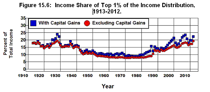
Source: The World Top Incomes Database.
It wasn’t until the government literally took over the economic system in 1942 and purchased the potential output that could not be sold to the private sector, given the distribution of income, that the unemployment problem was solved as the system was brought to full capacity. And it wasn’t until after the non-federal debt ratio and the level of income concentration fell during the war—and as the income concentration continued to fall after the war—that the domestic mass markets needed to sustain mass production were able to grow at the pace needed to maintain full employment in the absence of speculative bubbles and dramatic increases in total debt.
Finally, it is worth emphasizing that the dramatic deleveraging of non-federal debt that took place from 143% of GDP in 1940 to 67% in 1945 took place within an environment in which total government expenditures had increased to 36% of GDP by 1945 and the rationing of consumer goods and strict controls on investment expenditures gave households and firms little choice but to pay down their debts as their incomes increased dramatically during the war. This feat was not accomplished through the magical powers of free markets to bring balance back into the economy through the liquidation of households and firms—the kind of liquidation that took place from 1929 through 1933 that drove the economy into the Great Depression of the 1930s.
World War II was hardly an optimal solution to the problems caused by the concentration of income and the overwhelming burden of debt created by the fraudulent, reckless, and irresponsible behavior of those in charge of our financial institutions in the 1920s. It should be obvious that it would have been better to have accomplished the same ends through a somewhat less massive government intervention in the economy to build up our public infrastructure by providing massive improvements in our transportation, public utility, and educational systems than by producing massive quantities of war materials.
All of these things should be obvious, yet, none of these lessons have been learned by the free-market ideologues whose only vision for the future is lower taxes, less government, deregulation, and paying off the national debt.
Endnotes
[15.1] High-Powered Money is estimated in Figure 15.2 by the sum of Total, Member-bank reserves from the Economic Report of the President 1960's Table D-42 and Currency outside banks from Table D-40. This sum underestimates the actual value of High-Powered Money in existence at the time by the amount of currency held in the vaults of banks since, as was noted in Chapter 6, vault cash was not considered to be part of reserves from 1917 until 1959. (Feinman)
[15.2] See the Appendix on Measuring Debt at the end of Chapter 3 for an explanation of the way in which the data from the Historical Statistics of the U.S., Federal Reserve Flow of Funds Accounts, and Bureau of Economic Analysis are used in this figure.
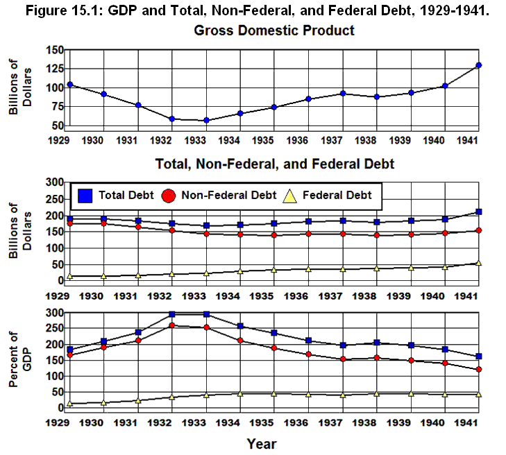
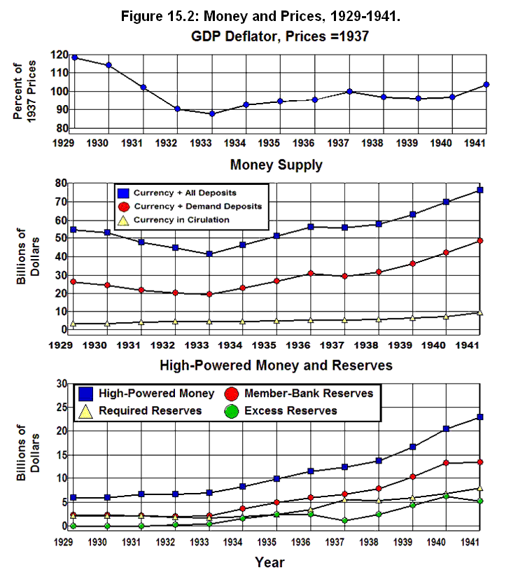
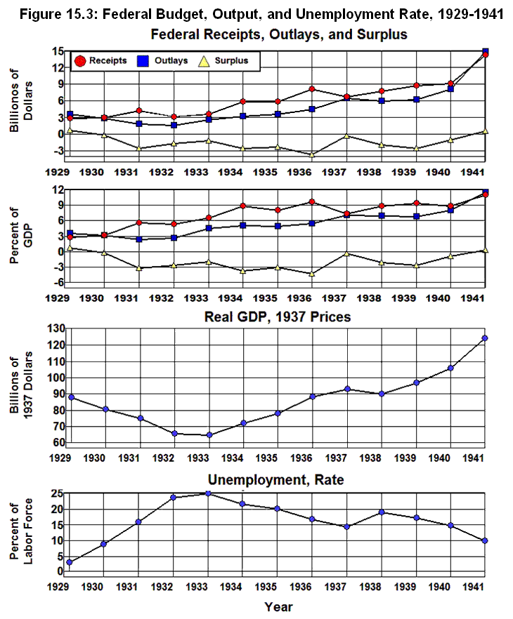
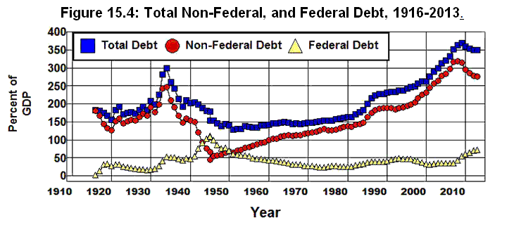
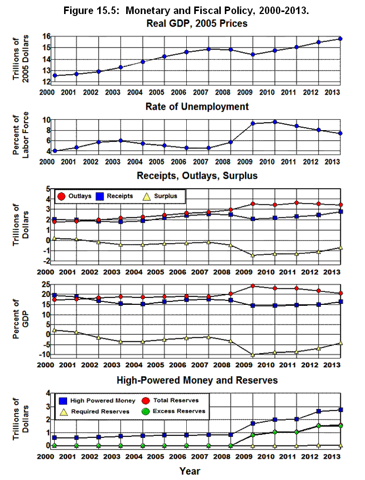
Where Did All The Money Go?
Chapter 16: Managing the Federal Budget
George H. Blackford © 2013, last updated 5/16/2014
It is fairly safe to say that the vast majority of the American people do not wish to cut Social Security or Medicare or those social-insurance programs that provide for the less fortunate among us. (Krugman) By the same token, it is reasonable to assume that the vast majority of the American people also want quality public education; effective public health programs;
safe streets and neighborhoods; a clean and safe environment; safe food, drugs, and other consumer products; safe working conditions; protection from predators who would fraudulently take advantage of them; fair and just legal and criminal justice systems; efficient public roads and highways; an effective national defense; and a stable, growing economy that is not plagued by cycles of booms and busts brought on by epidemics of recklessness and fraud in our financial system that drive our country and people deeper and deeper into debt and lead to the kind of economic catastrophe we are in the midst of today. (Amy)These are the kinds of things that only government can provide, but, unfortunately, there is a problem: For government to provide these things they must be paid for, and as we saw in Chapter 11, for much of the past thirty years we have failed to do so as is indicated by the way in which federal debt has increased relative to GDP since 1980. As we will see in Chapter 17, this problem is particularly challenging in light of the strain on the federal budget expected to occur as the baby boomers retire and expenditures on Social Security and Medicare increase. This chapter examines the nature of the choices involved in coming to grips with this problem.
Summary of the Federal Budget
Many people believe we can reduce the federal budget by a significant amount, by 10%, for example, without cutting defense or Social Security or Medicare and without decimating those programs that make up our social safety net simply by cutting the rest of the government. At the same time, there are those at the other end of the political spectrum who believe all we have to do to solve our fiscal problems is cut defense. What do we find when we look at the actual numbers in the federal budget?
Figure 16.1 is constructed from the OMB's Table 3.1—Outlays by Superfunction and Function. This figure plots a breakdown of the actual expenditures of the federal government in terms of its three largest categories (Superfunctions) from 1940 through 2012—Defense, Human Resources, and Net Interest—plus All Other Outlays which is calculated by subtracting the sum of the the three largest categories from Total Outlays.
Source: Office of Management and Budget. (3.1 10.1)
The first thing we see when we look at the graphs in this figure, just as we saw when we looked at similar graphs in Figure 13.2, is that even though the size of the federal budget has changed very little relative to the economy since the 1950s, the Human Resources component of the budget—those programs that make up our social-insurance system including Social Security, Medicare, and those programs that provide for the less fortunate among us—has grown dramatically. It has gone from less than 20% of the budget in the early 1950s to more than 60% in the 2000s. At the same time, Defense has decreased just as dramatically, going from over 60% of the budget to around 20%.
Meanwhile the third largest category, Net Interest, reached a high of 15.4% of the budget in 1996, and it stood at 8.7% of the budget in 2007 (the year before the federal budget was distorted by the financial panic in 2008 and the economic crisis that followed).
When we look at the rest of the government we find that All Other Outlays has gone from a high of 23.0% of the budget in 1950 to a low of 5.2% in 1954 (and 2010), and it stood at 6.7% in 2007.
Human Resources in Figure 16.1 is broken down in Figure 16.2. This figure is constructed from the OMB's Table 11.3—Outlays for Payments for Individuals and breaks down the Human Resources portion of the budget into four components: The first, Retirement/Disability, is the sum of all federal expenditures on retirement and disability programs listed in Table 11.3. The second, Healthcare, is the sum of all federal expenditures on healthcare listed in Table 11.3. The third, Other Payments for Individuals, is the sum of all federal expenditures on all payments-for-individual programs listed in Table 11.3 that are not medical or retirement/disability programs. The final component, Other Human Resources, is the total of all government expenditures on all other Human Resources programs and is constructed by subtracting the sum of the other three components in Figure 16.2 from Human Resources in Figure 16.1.
Source: Office of Management and Budget. (11.3 3.1 10.1)
When we look at the breakdown in Human Resources in Figure 16.2 we find that, while there were significant increases in all the graphs in this figure from 1965 through 1975, only Healthcare continued to rise after 1975. Healthcare grew almost continuously, from virtually nothing in 1965 to the point where it rivaled Retirement/Disability as the largest component of Human Resources in 2009. This graph makes it clear that rising healthcare expenditures is the most challenging problem in the federal budget. Healthcare is rapidly becoming the largest component of Human Resources which, in turn, is the largest component in the total budget.
What do we find when we look for savings in each of the separate categories in these two figures?
Net Interest, All Other Outlays, and Defense
Net Interest in Figure 16.1 must be paid when it comes due, so nothing can be saved there.
As for All Other Outlays in Figure 16.1, this category is constructed by subtracting the sum of Defense, Human Resources, and Net Interest from Total Outlays. It shows us how much the federal government spent on everything else the government does. All Other Outlays consists of such things as expenditures on Energy, Natural Resources and Environment, Transportation, Community and Regional Development, International Affairs, General Science, Space, Technology, Agriculture, Administration of Justice, General Government, and everything else the federal government does.
It is obvious—or at least it should be obvious to anyone who looks at the actual expenditures of the federal government in this category plotted in Figure 16.1—that there is no reason to believe we can save a substantial amount of money by cutting All Other Outlays without substantially inhibiting the government's ability to function. The expenditures on programs in this category have already been cut by over 50% relative to the economy since 1980, and even if we were to eliminate all of these expenditures completely—which, of course, we can't do and still have a functioning government—we would succeed in reducing the size of the federal budget by less than 7%.
As for Defense, It is apparent from Figure 16.1 that there may be room to make additional cuts in the area of Defense. After all, in 2007, Defense was barely below where it stood in 1980 (20.2% versus 22.7% of the budget and 4.9% versus 3.9% of GDP) when we were still waging the Cold War against the Soviet Union. With the end of the wars in Iraq and Afghanistan there may be room to maneuver here. Just the same, there is no reason to believe we can solve all of our fiscal problems simply by cutting Defense. Even if we were to cut Defense in half—which few people would be willing to do—it would only reduce the total federal budget by about 10%.
Thus, if we are serious about saving as much as 10% of our total federal taxes, unless we are willing to cut Defense by 50%, we must look to Human Resources. That's where the money is, and it's also where Social Security and Medicare are, as well as the other social-insurance programs that make up our social safety net. The question is: Does it really make sense to think we can save a lot of money by cutting Human Resources without cutting Social Security or Medicare and without cutting other programs that make up our social safety net?
Human Resources
It is clear from Figure 16.2 that Retirement/Disability and Healthcare combined dominate Human Resources as they accounted for some 84% of all Human Resources expenditures in 2007. This would suggest that if we are to find ways to make substantial cuts in Human Resources we should begin by looking at Retirement/Disability and Healthcare.
Retirement/Disability
Table 16.1 shows all of the federal programs listed in the OMB's Table 11.3 that are included in Retirement/Disability in Figure 16.2 along with the amount spent on each program in 2007, the percent of GDP each program consumed in that year, and the percent of the federal budget each program consumed as well.
Table 16.1: Expenditures Included in Retirement/Disability, 2007.
Program (2007) Billions of Percent of Percent of Dollars GDP Budget Social security and railroad retirement: 586.7 4.10% 21.50% Social security: old age and survivors insurance 483.3 3.37% 17.71% Social security: disability insurance 97.5 0.68% 3.57% Railroad retirement (excl. social security) 5.8 0.04% 0.21% Federal employees retirement and insurance: 138.0 0.96% 5.06% Military retirement 43.5 0.30% 1.59% Civil service retirement 60.9 0.42% 2.23% Veterans service-connected compensation 31.1 0.22% 1.14% Other 2.6 0.02% 0.10% Public assistance and related programs: 36.3 0.25% 1.33% Supplemental security income program 32.9 0.23% 1.21% Veterans non-service connected pensions 3.4 0.02% 0.12% Total: Retirement/Disability
761.0 5.31% 27.89% Source: Office of Management and Budget. (11.3 3.1 10.1)
It is clear from this table that Retirement/Disability is dominated by Social Security in that fully 76% of the total in 2007 went to Social Security where 20% went to civil service, military, and railroad retirement/disability programs, and 4% went to the Supplemental Security Income (SSI) program. It is equally clear from this table that there is no way to make substantial cuts in this portion of Human Resources without cutting Social Security. After all, military, civil servants, railroad employees, and other government employees are just as entitled to their retirement/disability benefits as are Social Security recipients.
This leaves the SSI program which was only 4% of Human Resource expenditures in 2007 and 1.2% of the entire federal budget. Aside from the fact that SSI was only 1.2% of the budget in 2007 and 0.23% of our gross income, as we saw in Chapter 14, SSI is the primary social safety-net program that provides for indigent disabled and indigent elderly individuals who are either not eligible for Social Security or whose benefits fall below a subsistence level. Not only would substantial cuts in this program save virtually nothing, they would tear a hole in our social safety net.
What about Healthcare?
Healthcare
Table 16.2 shows all of the federal programs listed in the OMB's Table 11.3 that are included in Healthcare along with the amount spent on each in 2007, the percent of GDP each program consumed in that year, and the percent of the federal budget each program consumed as well.
Table 16.2: Expenditures Included in Healthcare, 2007.
Program (2007) Billions of Percent of Percent of Dollars GDP Budget Medicare: 435.0 3.04% 15.94% Medicare: hospital insurance 204.9 1.43% 7.51% Medicare: supplementary medical insurance 230.1 1.61% 8.43% Medicaid 190.6 1.33% 6.99% Children's health insurance 6.0 0.04% 0.22% Veterans: 38.1 0.27% 1.40% Hospital and medical care for veterans 30.5 0.21% 1.12% Uniformed Services retiree health care fund 7.6 0.05% 0.28% Other Medical Care: 12.6 0.09% 0.46% Indian health 3.3 0.02% 0.12% Health resources and services 5.9 0.04% 0.22% Substance abuse and mental health services 3.2 0.02% 0.12% Other 0.3 0.00% 0.01% Total: Medical care 682.4 4.76% 25.01% Source: Office of Management and Budget. (11.3 3.1 10.1)
Here we are looking at 25% of the budget. It is clear from this table that Medicare and Medicaid dominate Healthcare in that these two programs accounted for over 90% of Healthcare expenditures in 2007 with Medicare accounting for 70% of that 90%. What about the 20% of this 90% that went to Medicaid?
Medicaid represented 7% of the federal budget and 1.3% of our gross income in 2007 and, again, as we saw in Chapter 14, Medicaid lies at the very core of our social safety net. According to the Census Bureau's Table 151. Medicaid—Beneficiaries and Payments: 2000 to 2009, some 75% of Medicaid's beneficiaries were either poor Children, indigent blind/disabled individuals, or indigent, elderly adults age 65 and over, and over 85% of Medicaid's expenditures went to these individuals. It would appear that there is very little room to cut here without causing a great deal of hardship and misery through the denial of medical services to poor children or indigent blind/disabled or indigent elderly adults.
That leaves the remaining 10% of the Human Resources budget that went to the other programs listed in Table 16.2. Here we are talking about 2% of the entire federal budget and 0.4% of our gross income in 2007. Of that 10%, 67.2% went to veterans (Hospital and medical care for veterans and Uniformed Services retiree health care fund), 10.6% to Children's health insurance, and 5.8% went to Indian health. Of the remaining 16.6%, 63.1% went to Health resources and services (a program that is designed to meet the healthcare needs in mostly rural underserved areas), 34.0% went to Substance abuse and mental health services (a program that is severely under funded given the extent of the substance abuse problem in our country), and 2.9% went to Other federal healthcare programs.
Veterans certainly have as much right to their medical benefits as Medicare recipients, so there is no reason to think we can or should cut veterans' medical benefits without cutting Medicare as well, and the rest of these programs play an important role in our social safety net. In addition, since the rest of these programs took up only 0.69% of the entire federal budget in 2007 and 0.13% of our gross income there is virtually nothing to be saved by eliminating these programs.
The leaves but two categories in Figure 16.2 to examine: Other Payments for Individuals and Other Human Resources.
Other Payments for Individuals
Other Payments for Individuals includes the expenditures on all of the federal programs in the OMB's Table 11.3 that are not medical or retirement/disability programs. The items included in this category along with the amount spent on each in 2007, the percent of GDP each program consumed in that year, and the percent of the federal budget each program consumed are given in Table 16.3.
Table 16.3: Non-Medical and Non-Retirement/Disability Programs, 2007.
Source: Office of Management and Budget. (11.3 3.1 10.1)
The first thing that jumps out from this table is that, in spite of the abundance of programs, we are talking about only slightly more than 9% of the entire federal budget here and less than 2% of our gross income.
While there were no programs that dominated this category, the ten largest items in Table 16.3 are arranged from largest to smallest and listed in Table 16.4. These ten items accounted for 93% of the total expenditures in the Other Payments for Individuals category in 2007.
Table 16.4: Ten Largest Items in Other Payments for Individuals, 2007.
Program (2007) Billions of Percent of Percent of Dollars GDP Budget Earned income tax credit 38.3 0.27% 1.40% SNAP (formerly Food stamps) (including Puerto Rico) 34.9 0.24% 1.28% Unemployment Assistance 33.2 0.23% 1.22% Housing assistance 33.0 0.23% 1.21% Student assistance—Department of Education and other 27.5 0.19% 1.01% Family support payments to States and TANF 21.1 0.15% 0.77% Payment where child credit exceeds tax liability 16.2 0.11% 0.59% Child nutrition and special milk programs 13.0 0.09% 0.48% Payments to States—Foster Care/Adoption Assist. 6.6 0.05% 0.24% Supplemental feeding programs (WIC and CSFP) 5.3 0.04% 0.19% Total: 10 Largest in Other Payments for Individuals 229.1 1.60% 8.39% As we saw in Chapter 14, the ten programs listed in Table 16.4 are the backbone of our social safety net. We're talking about the Earned income and Child Tax Credits (22% of Total: Other Payments for Individuals in Table 16.3) that are designed to encourage work and assist the working poor who pay over 14% of their earned income in payroll taxes. About Food Stamps, Child nutrition, Special milk, and Supplemental Feeding program (22%) that assist the poor in feeding themselves and their children. About Student Aid (13%), Unemployment Compensation (26%), and about Foster Care and Adoption (2.6%). And we're talking about only 9% of the entire federal budget in all of the programs in Other Payments for Individuals combined and less than 2% of our gross income.
There is is no reason to think that we can obtain a great deal of savings by making substantial cuts in this portion of the budget without dismantling our social safety net and causing a great deal of hardship and misery. The money just isn't in these programs, and it's through these programs—combined with Medicaid and SSI—that our war against hardship and misery is waged.
Other Human Resources
This leaves only Other Human Resources in the Human Resources portion of the budget. Other Human Resources is the total of government expenditures on all Human Resources programs that are not included in the other categories in Figure 16.2. This residual can be disposed of rather quickly. It represented only 2.8% of the budget in 2007 and less than 1% of our gross income, and, aside from the fact that 2.8% of the budget is insignificant in the grand scheme of things, as is shown in Figure 16.2, this portion of the budget has already been cut by almost 50% since 1980. There is no reason to believe that substantial additional cuts can be found here.
Waste, Fraud, and Abuse
There are widespread complaints about waste, fraud, and abuse in the federal budget, and there is always reason to strive for improvement in this area. At the same time, there is little reason to believe our efforts in this regard can have much of an effect on the size of the budget. Waste, fraud, and abuse just aren't that important in the grand scheme of things when it comes to the size of the budget.
Defense and Healthcare
As was noted above, Defense in Figure 16.1 is barely below where it stood in 1980s when we were still waging the Cold War against the Soviet Union. It may be reasonable to assume that through realigning our budget priorities away from the military threats we faced twenty-five or thirty years ago and toward those we face today it may be possible to eliminate some waste in the defense budget as we demobilize from the Iraq and Afghanistan wars. It was also noted above, however, that in order to cut the total budget by 10% in this way we would have to cut Defense by 50%, and virtually no one is willing to cut the defense budget by this amount.
And then there’s Healthcare.
According to the Organization for Economic Cooperation and Development (OECD) and Central Intelligence Agency World Factbook, we not only spent more per person and as a percent of GDP on healthcare in 2010 than any other country in the world, and we spent more than twice as much per person as the average of the other OECD countries ($8,233 compared to $3,153) and almost twice as much as a percent of our gross income (17.6% compared to 9.4%). And, yet, we ranked 24th among the 34 OECD countries in terms of life expectancy (51st among all countries) and 28th among these 34 countries in terms of infant mortality (50th among all countries).[16.1]
In other words, even though we spend more on healthcare than any other country in the world, and spend twice the average of what the other OECD countries spend, we benefit less from our expenditures than most of the OECD countries benefit from theirs in that their people live longer than we do, they are healthier than we are, and the rate at which their children die in infancy is less than the rate at which out children die in infancy. (OECD OECD Charts NYT IOM JAMA1 JAMA2) There is obviously something wrong here!
Both private and public healthcare costs in the United States have increased dramatically over the past twenty years, and even though the Affordable Care Act promises to improve the health of our population by increasing the availability of healthcare, there is little reason to believe this act will lead to substantial savings to taxpayers in the absence of a public option. It is either a public option or some other kind of single-payer mechanism that makes it possible for healthcare costs to be controlled in those countries that have better health statistics than we do, and there is little reason to believe we will be able to control our healthcare costs, and, at the same time, maintain the health of our population until we implement a similar system at home.
It is also worth noting that, even though cleaning up our healthcare mess by adopting a public option or implementing some other kind of single-payer mechanism will undoubtedly save taxpayers money, it will not necessarily reduce the size of the federal budget or lead to lower taxes as the availability of healthcare is expanded within the population. Depending on the kind of single-payer option implemented, the savings to taxpayers could be accomplished through a net savings in the combined private and public costs of healthcare as private healthcare costs fall by more than public healthcare costs go up.
Defense and Healthcare made up 45% of the federal budget in 2007, and, as has been indicated, there may be room for significant reductions in waste in these areas through 1) realigning our defense priorities as we demobilize in response to the end of the wars in Iraq and Afghanistan and 2) making our healthcare system more efficient by implementing a single-payer system. At the same time, there is no reason to believe we can reduce the total federal budget significantly by simply eliminating specific instances of waste, fraud, and abuse in these portions of the budget in spite of the fact that, on rare occasions, these instances run into the hundreds of millions or even billions of dollars. (Coburn Sanders MFCU NYT)
Specific Instances of Waste, Fraud, and Abuse
The fundamental problem with Defense is to be found in bad policy decisions that misalign our budget priorities, and the fundamental problem with Healthcare is our over-reliance on a private, corporate-oriented, multiple-payer, third-party, fee-for-service payment system that makes it impossible to produce optimal healthcare outcomes at a reasonable cost. Specific instances of waste, fraud, and abuse are trivial in comparison to the systemic problems in Defense and Healthcare. The numbers just don't add up.
Even if we can find specific instances that cost the government as much as a million dollars or more, we can't cut the federal budget by as much as 10% by saving as little as one million dollars at at time. The federal budget was $3,455 billion in 2013. Ten percent of that is $345.5 billion. That's 345,500 millions! That means that in order to reduce the budget by 10% one million dollars at a time we would have to find 345,500 instances in which one million dollars worth of waste, fraud, or abuse occurs. We can’t even count to 345,500 let alone find 345,500 ways in which the federal government squanders one million dollars on an annual basis. Even trying to cut the budget by as little as 1% in this way would require finding 34,505 such instances.
When we look at the way the federal budget is actually spent in the real world, these numbers become even more problematic. Retirement/Disability, Healthcare, and Other Payments for Individuals make up over 60% of the budget. While there may be some inefficiencies in the administration of the programs in these categories of the budget, administrative costs are relatively insignificant compared to the benefits these programs pay out. Medicare's administrative costs, for example, are as little as 2% of the benefits it pays out and Social Security's as little as 1%. Medicare and Social Security alone took up 37% of the total budget in 2007, and even if we were to eliminate all of their administrative costs it would reduce the total budget by less than 1% (0.02 x 0.37 = 0.0074).
This means that in order to find significant amounts of waste, fraud, and abuse in this 60% of the budget we have to look at the tens of millions of beneficiaries whose benefits average in the thousands of dollars. Now we are talking about the need to find millions of instances of waste, fraud, and abuse in the thousands of dollars range, not just hundreds of thousands in the millions of dollars range.
There is no way we can expect to do this without expanding the size of the federal bureaucracy, and since it costs money to expand the federal bureaucracy, there is no guarantee we will be able to reduce the budget at all by doing this even if by doing this we are able to eliminate all of the waste, fraud, and abuse that may exist among the tens of millions of beneficiaries these programs serve. It may even cost more to expand the bureaucracy than can be saved. (Lindert) This is especially so in light of the fact that there doesn't seem to be any reason to believe that waste, fraud, and abuse is very widespread among these beneficiaries in the first place.
The nature of this problem can be seen by examining a report published by the Federal Reserve Bank of St. Louis in which it estimated that some $3.3 billion worth of fraudulent unemployment compensation claims were paid in 2011. That works out to 3.06% of the total $108 billion worth of claims that were paid out in 2007 in a program that had 3.7 million beneficiaries in that year. The point is that we can't simply eliminate this $3.3 billion worth of fraudulent unemployment compensation claims by waving a wand or by increasing the amount of money we spend to investigate those few who are actually committing this fraud, 88,000 of which were collecting benefits while working part time and being paid under the table. We have to investigate all of the 3.7 million beneficiaries in order to find those few, and this can't be done without paying people to do it.
Since the $108 billion in unemployment compensation claims amounted to only 3.00% of the $3,603 billion federal budget in 2011, and only 3.06% of this 3.00% of the federal budget was wasted in specific instances of fraud in 2011, that works out to 0.09% of the entire federal budget that was wasted in fraudulently collected unemployment claims in 2011 (0.0306 x 0.03 = 0.000917).
This means that even if we are successful in eliminating all of the $3.3 billion in fraudulent unemployment compensation claims in the system, the most we can save by doing this is less than 0.09% of the total budget, and if it costs us more than $3.3 billion to expand the bureaucracy in order to eliminate this 0.09% of the total budget it will actually cost us more to eliminate this fraud than we can save. It also means that if we were to find similar rates of fraud (3.05%) in the rest of the 60% of the budget taken up by Retirement/Disability, Healthcare, and Other Payments for Individuals, the most we can save by eliminating this fraud is 1.8% of the total budget (0.0305 x .60 = 0.0183), and if it costs us more than $108 billion (0.0305 x 3,5237 = 107.8785) to expand the bureaucracy in order to do this, it will cost us more than we can save.
This doesn't mean we shouldn't try to eliminate waste, fraud, and abuse in this portion of the budget wherever and whenever we can. It only means we should not expect to be able to save $108 billion or reduce the federal budget by as much as 1.8% as a result of our efforts to do so.
As for the rest of the budget, there is no reason to believe significant savings can be found there either. We have already discussed Defense—fraud or no fraud, virtually no one is willing to cut defense by a sufficient amount to make a significant difference in the size of the total budget—and, as was noted above, Net Interest must be paid when it comes due so nothing can be saved there. As was also noted above, All Other Outlays in Figure 16.2 has already been cut by almost 50% since 1980 and Other Human Resources in Figure 16.3 by more than 50%. The programs in these last two categories take up less than 10% of the total budget, and since they have been cut so dramatically over the past thirty years, there is no reason to think we can save a substantial amount by cutting this 10% of the budget even further.
That's all there is in the rest of the budget! Defense, Net Interest, and All Other Outlays in Figure 16.2 plus Retirement/Disability, Healthcare, Other Payments for Individuals, and Other Human Resources in and Figure 16.3 make up the entire federal budget. Everything in the budget on which the federal government spends money is included in one or another of these seven categories.
Finally, I would note a headline that recently appeared in Bloomberg News, Millionaires Got $80 Million in Jobless Aid in Recession, that further highlights the nature of the problem faced by those who think our fiscal problems can be solved by eliminating specific instances of waste, fraud, and abuse in the federal budget. According to the author, Frank Bass:
The $80 million represents less than 0.01 percent of this year’s $845 billion projected deficit. Yet the unemployment aid to millionaire households underscores the lack of means-testing in some federal aid programs . . .. The aid also is a reminder of the difficulty of reining in spending.
The fact is, some 35% of that $80 million was recouped in income taxes on those benefits, only $52 million was kept by the recipients, and that $52 million is not only less than 0.01% of the $845 billion projected deficit (52/845,000 = 0.0000615), it is less than 0.002% of the $3,537 billion federal budget in 2012 (52/3,537,000 = 0.0000147).
In addition, it is a mistake to think we can reduce the budget by even this piddling amount by converting our unemployment insurance program into a means-tested welfare program since this ignores the added cost of the increased bureaucracy it would take to investigate the income status of the millions of beneficiaries in this program. By simply making unemployment benefits available to all who pay into the system, irrespective of income, those bureaucratic costs are avoided, and the efficiently with which payments can be made to the unemployed is increased dramatically. (Lindert)
But the real absurdity here is the delusion that this $52 million has something to do with the $845 billion projected deficit or the difficulty of reining in spending in a $3,537 billion budget: What is the point in wasting time and energy discussing the fate of $52 million within the context of an $845 billion deficit and a $3,537 billion budget? That's like worrying about $52 when your total expenses are $3,537,000 and you are $845,000 in the hole. Even if we could reduce the deficit $52 million a day by concerning ourselves with this sort of nonsense it would take 44.5 years to solve a $845 billion deficit problem in this way (845,000 / 52 / 365.25 = 44.4901). This is the epitome of what it means to be penny wise and pound foolish.
Summary of Waste, Fraud, and Abuse
In searching for ways to cut the federal budget it is important to understand that cutting a small amount from a large portion of the budget or a large amount from a small portion of the budget may yield a lot of money in absolute terms, but it doesn't yield a lot of money relative to the size of the total budget. It only reduces the total budget by a small amount. To reduce the total budget by a large amount we have to cut a large amount from a large portion of the budget. That's just grade school arithmetic.
When we look at the actual expenditures in the federal budget over the past forty years we find that it is not possible to cut a large amount from a large portion of the budget without cutting defense, Social Security, Medicare, or the programs that make up our social safety net because that's where the money is. The rest of the budget has already been cut to the bone since 1980, and there simply isn't enough money in the rest of the budget to make a difference even if we cut a large amount from this small portion of the budget.
We also find that even though there may be substantial savings to be found in realigning our defense priorities as we demobilize from the Iraq and Afghanistan wars and by reorganizing healthcare into a single-payer system, there is no reason to believe we would be able to reduce the size of the total budget by a substantial amount even if we were to realize these savings. We would have to cut the defense budget in half in order to reduce the total budget by 10% in this way, something which virtually no one is willing to do, and, depending on the kind of single-payer option implemented, implementing a single-payer system in order to improve the efficiency of our healthcare system could require an increase the size of the federal budget rather than a decrease.
At the same time, we find that there is no reason to believe we can reduce the size of the federal budget by increasing our efforts to target specific instances of waste, fraud, and abuse. There simply aren't enough specific instances of waste, fraud, and abuse in the budget that are of sufficient magnitude to make a difference in this regard. At best, all we can hope to do by expanding our efforts in this area is cut a small amount from a large portion of the budget, and doing this could actually cost us more to do than we can save by doing it. (Lindert) As was noted above, this does not mean we should ignore this problem. It only means that we should not expect to see a substantial reduction in the size of the budget as a result of our efforts to solve it. Those who think otherwise have a problem with arithmetic. Their numbers just don't add up. (Coburn Sanders MFCU NYT StLuisFed)
Realigning our defense priorities away from the threats we faced twenty-five or thirty years ago and toward the threats we face today, reorganizing healthcare toward a single-payer system, and targeting specific instances of waste, fraud, and abuse within the budget are the most efficient, least harmful, and only sensible ways to address the problem of waste, fraud, and abuse in the federal budget. Attempting to address this problem by simply cutting the budget—which is what we have been trying to do over the past thirty years—is a recipe for disaster.
When we realign our defense priorities, reorganize our healthcare system, and target specific instances of waste, fraud, and abuse we affect the lives of relatively well off or undeserving individuals who can, more or less, take care of themselves. As a result, we don’t have to worry about increasing malnutrition and death rates among poor children or indigent disabled/elderly adults or about forcing people who can’t find work—for whatever reason—to become desperate which is what we can expect when we simply cut the funds to those programs contained in Other Payments for Individuals in Figure 3. We also don't have to worry about impairing the government’s ability to protect the public from poisonous food, dangerous drugs, harmful consumer products, fraud and predatory practices in our financial system, unsafe work environments, potential environmental catastrophes or to maintain our transportation systems and educate our population which is what happens when we arbitrarily cut funds to those programs contained in All Other Outlays in Figure 16.2. (Amy Lindert)
Making the Government Fiscally Sound
A fundamental, real-world truth that has been almost completely ignored in the otherwise hopelessly irrational debate we have been subjected to over the past forty years is that there are certain things that only the government can do. One is provide a system of national defense. Another is provide legal and law enforcement systems that set and enforce the rules in a fair, efficient, and effective way. Another is provide the public education and infrastructure that makes possible such things as an educated labor force and an efficient transportation system. Yet another is to provide a social insurance system that makes possible such things as unemployment insurance, efficient healthcare and retirement systems, and a welfare system, all of which provide ordinary people some insurance against the devastation caused by the vagaries of our economic system. (Amy Lindert)
It seems to me quite clear that these are all things that the vast majority of the people want the government to provide for them. This does not mean the vast majority of the people are moochers who expect the government to take care of their every need. It means the vast majority of the people realize that, in the real world, only the government can provide these kinds of economic goods in a fair, efficient, and effective way. These are not the kinds of economic goods that can be provided fairly, efficiently, or effectively by the private sector of the economy.
The response from those who are waging their own private war against the federal government is that 1) reorganizing our healthcare system to include a public option is socialism, 2) the world is too dangerous to cut defense, and 3) we must cut the rest of the budget—especially Social Security and Medicare—because deficits and the national debt are out of control.
But in the real world, even if we are not willing reorganize our healthcare system or cut defense, solving our deficit and debt problems without cutting the rest of the budget is not all that complicated. All we have to do to balance the budget without cutting defense or our social-insurance programs is increase taxes.
On Increasing Taxes
Many people believe that Americans are terribly overtaxed—that we can't afford the tax increases needed to fund the federal government. This belief doesn't hold up to even a casual look at the numbers. Table 16.5 shows how the United State's ranking among the 34 OECD countries has changed since 1980 in terms the percentage of gross income (GDP) paid in taxes.
Table 16.5: OECD Countries that Pay Less Taxes than We Do
Percent of GDP, 1980-2010.
1980
1990
2000
2005
2010
USA
26.4
Japan
28.6
Spain
34.3
Portugal
31.1
Portugal
31.3
Australia
26.2
Australia
28.0
Portugal
30.9
Ireland
30.1
Greece
30.9
Japan
24.8
USA
27.4
Australia
30.4
Australia
30.0
Switzerland
28.1
Switzerland
24.6
Portugal
26.8
USA
29.5
Switzerland
28.1
Japan
27.6
Spain
22.6
Greece
26.4
Switzerland
29.3
Japan
27.3
Turkey
25.7
Portugal
22.2
Switzerland
24.9
Japan
26.6
USA
27.1
Australia
25.6
Greece
21.8
Korea
19.5
Turkey
24.2
Turkey
24.3
Korea
25.1
Korea
17.1
Chile
17.0
Korea
22.6
Korea
24.0
USA
24.8
Mexico
14.8
Mexico
15.8
Chile
18.9
Chile
20.7
Chile
19.6
Turkey
13.3
Turkey
14.9
Mexico
16.9
Mexico
18.1
Mexico
18.8
Source: Organization for Economic Cooperation and Development, Comparative Tables.
We have moved from tenth from the bottom on this list to third from the bottom over the past thirty years. Among the advanced countries of the world, only Chile and Mexico paid less in taxes as a percent of their gross income than we did in 2010. There is no reason to believe we can't afford the taxes needed to fund Social Security, Medicare, and the rest of the federal government even if we are not willing to cut defense or reorganize our healthcare system.
In principle, at least, it is not that difficult to make the government fiscally sound. This could be accomplished quite easily by
rescinding the 2001-2003 Bush tax cuts,
eliminating unwarranted tax deductions and credits, and especially the special treatment of capital gains and dividends,
increasing the top marginal tax rates, (Fieldhouse Diamond Sides) and
increasing taxes on corporations.
Dividends, Capital Gains, and the Top Marginal Rates
We had a surplus equal to 2.3% of GDP in 2000 before the 2001-2003 tax cuts. Does it really make sense to dismantle the federal government and make dramatic cuts in Social Security and Medicare rather than rescind those cuts? It's just common sense that if we want to solve our deficit/debt problem and maintain our social-insurance programs with a functioning government, the place to begin is by rescinding those tax cuts.
In addition, as we saw in Chapter 14, the special treatment of dividends and capital gains led to a $118.8 billion subsidy for the top 1% of the income distribution in 2007—an average government subsidy of $73,903 per household for the top 1%. There is absolutely no economic, ethical, or moral justification for this kind of subsidy, especially in the midst of the kind of fiscal crisis we will face in the future as the baby boomers retire if we don't raise taxes.
Eliminating the special treatment of dividends and, especially, capital gains, when combined with a substantial increase in the top marginal tax rate will have the added benefit of reducing the potential gains that can be reaped from the kinds of fraudulent, reckless, and irresponsible behaviors on the part of those who run our financial institutions that created the economic catastrophe we are in the midst of today. This will reduce the single most powerful incentive that motivates these kinds of behaviors. It will also have the effect of strengthening our mass markets to the extent it reduces the need to increase taxes on the rest of the income distribution and, thereby, help to maintain the domestic purchasing power of the vast majority of the population that is essential to maintaining our domestic mass markets. (Fieldhouse Diamond Sides)
On Taxing Corporations
When it comes to the need to increase taxes on corporations, it is worth emphasizing that corporations consume government services far beyond those consumed by other businesses. Corporations dominate our legal and law enforcement systems where lawsuits brought to settle disputes between corporations or between corporations and their customers, their employees, or the government clog up our courts.
Corporations benefit massively from the government’s providing and enforcing copyright and patent protections and from the limited liability protection provided to corporations by the government. Corporations also benefit massively from our public transportation systems and from the educated workforce our public education systems provide, and a major reason our defense budget is so large is to protect the foreign interests of American corporations throughout the world.
There are reasons why international corporations locate in countries whose governments provide highly developed legal, law enforcement, transportation, public education, and national defense systems. (Amy Lindert) Why should corporations be given a free ride as ordinary people and other forms of business organization are taxed to pay for the government services corporations disproportionately consume and from which corporations derive such massive economic benefits?
Those who wish to eliminate the corporate profits tax argue this tax is somehow unfair because it taxes income twice—once when it is earned by the corporation and a second time when it is received by stockholders in the form of dividends. This is a fallacious argument. To begin with, not all profits are paid out in dividends. More to the point, however, is the fact that all taxes come out of profits, not just a tax on profits.
A corporation subject to a 50% corporate profit tax on a $10 million before tax profit generated from $100 million in sales would have the same after tax profit as a corporation in the same situation that paid no corporate profit tax but, instead, paid a 5% sales tax, a $5 million property tax, or a $5 million dollar tax of any other kind. In any of these situations the corporation would have the same $5 million after tax profit. Why does it make sense to consider a corporate profit tax to be a double taxation of income in this situation but not an alternative tax? There is, of course, a semantic difference here but not a real difference.
The bottom line is that the same after tax profit is received by the corporation and stockholders irrespective of the kind of tax paid. A corporate profits tax is a cost of doing business, just like any other tax, and the notion that it somehow unfair because it leads to a double taxation of income and other taxes do not is nonsense.
The corporate profits tax is actually a less onerous tax than most since it is paid only when there is a profit. It is not paid during hard times when there are no profits and funds are scarce, or by owners of startup companies that have to make investments before they can make a profit and are forced to take losses as they build their businesses. Alternative taxes must be paid during hard times and by startup companies whether there are profits or not. As a result, the corporate profits tax is a much more business friendly tax than other taxes since it makes it easier for existing corporations to survive during hard times and for investors to start new corporations. In this sense, a corporate profits a tax is much fairer than other taxes.
It is argued that since other countries have lower corporate taxes, if we don’t cut our taxes corporations will relocate to countries with lower taxes and we will lose jobs, but this is only a problem because we allow corporations that locate in countries that serve as tax havens free access to American courts and markets. Corporations that locate in tax havens should be forced to pay a compensating tax to the American government in order to access our courts and markets. Not only would such a tax save jobs by preventing corporations from relocating, it would force corporations to pay their fair share for the government services they demand and on which their very existence depends. It would also help to make it possible to rebuild and maintain the public infrastructure and social capital provided by the government that is essential to obtaining and maintaining economic prosperity. (Amy) What's more, failing to tax corporations has ominous implications for the future.
For the past sixty years, American corporations have been able to minimize their contribution toward paying for the government services they consume within the United States by migrating or threatening to migrate from high tax states to low tax states as they play one state off against another to obtain lower taxes. This has led to short-term economic benefits to corporations and to low-tax states as people in the high-tax states that provide better public services follow the jobs created by corporations in the low-tax states that provide inferior public services, especially education. It has also shifted the burden of paying for government services, especially education, away from those who benefit from these services the most—people in the low-tax states to which the corporations and the people who are educated in the high-tax states migrate—on to the backs of those who benefit from them the least—the people in the high-tax states who are unable to migrate and who are loosing their tax base to the low-tax states.
The long-term nature of this effect has been particularly dramatic in the area of education where the private cost of higher education has increased to the point where student debt today is larger than either credit card or automobile debt. In 1970 the United States led the world in the percent of young adults with a college degree. By 2011 we had fallen to 16th place. Instead of educating our own to meet the needs of corporate America, as corporate taxes fell and American educational standards lagged behind, American corporations have begun to rely on foreigners to fill their ranks in those jobs that require higher education—especially in math, the sciences, and engineering—and an ever increasing number of positions at our colleges and universities are being filled by foreign students. If this trend is allowed to continue to its logical conclusion we will evolve into a society in which only the children of the wealthy are able to afford a quality education, and the quality and productivity of our labor force will fall.
Forcing countries to compete for corporate favors by lowering taxes is no different than forcing states to compete in this way, and there is no reason to expect the results to be different if this drama is allowed to play itself out on the world stage than they have been as it has played itself out on the national stage within the United States over the past sixty years. There will be economic benefits to corporations and low tax countries in the short run, but, in the long run, government services will deteriorate throughout the world, and, in the end, there will be a loss in economic and social wellbeing for the vast majority of the world’s population. What’s more, we can expect the losses to be greatest in those countries, such as the United States, that have the most to lose. (Rodrik)
Maintaining Public Infrastructure and Social Capital
For thirty-five years following World War II our government made huge investments in our society. It built our Interstate Highway System. It made huge investments in our educational system through such programs as the GI Bill and National Defense Education Act as it subsidized the education of the best and the brightest among us who, in turn, provided the scientific research that led to the tremendous advanced in technology we have seen since World War II. It also made huge investments in our social-insurance system. The end result of these public investments was a highly educated and productive labor force, a tremendous increase in our public infrastructure, and a social environment that made it possible for our economic system to flourish.
It also made it possible for those who benefited the most from the socioeconomic environment created by the stability of our government to amass huge fortunes. If our economic system is to continue to flourish the government and the social capital that made this possible in the past must be maintained, and it cannot be maintained if those who benefit the most from our government do not pay back enough to keep that government functioning to maintain the public infrastructure and provide the social environment that made their prosperity possible.
Since 1980 we have lowered taxes on the wealthy and increased taxes on the not so wealthy as we dismantled our regulatory systems and cut back on other government programs that serve the common good and promote the general Welfare within our society. The result has been a growing divisiveness within our society and economic stagnation for the vast majority of our population as we have fallen behind in educating our children, our public infrastructure has deteriorated, the rate of increase in productivity has fallen, and fraud has run rampant in our financial system leading to the worst economic disaster since the Great Depression.
If those who benefit the most from our economic system do not pay back in taxes enough to rebuild the public infrastructure and social capital they consumed in the process of reaping the benefits they have gained from our economic system, there is little hope for the future, and it is important to note that this does not mean just the top one or two percent of the income distribution must pay back. It means that everyone who is capable of making a contribution toward this end must do their part. (Fieldhouse Diamond Sides) If this is not done we will consume the public resources that were left for us by previous generations, and in failing to replenish those resources, we will limit the economic possibilities for future generations.
Rescinding the Bush tax cuts, treating capital gains and dividends as ordinary income, and increasing the top marginal tax rates and taxes on corporations would not necessarily give us a surplus today, but it would at least give us a tax structure that is viable. If these actions were to be combined with an increase in government expenditures to rebuild our public infrastructure and enhance the educational opportunities available to our children, there is every reason to believe it would not only increase the rate of productivity growth and help to solve our unemployment problem, it would also stabilize the federal debt relative to GDP as well, just as similar policies stabilized the debt relative to GDP in the 1930s. It would also make it possible to pay for the government services the people demand, such as Social Security, Medicare, and the rest of our social-insurance system without having to dismantle that system.
It is the foolish belief that we can have good government and all of the essential services and benefits that only government can provide without paying the taxes necessary to provide these services and benefits that has led us to where we are today. The only way we can have these essential services and benefits is by strengthening the institutions that provide them, and the only way we can strengthen those institutions is by raising the taxes needed to provide the government services and benefits people demand: quality public education; effective public health programs; safe streets and neighborhoods; a clean and safe environment; safe food, drugs, and other consumer products; safe working conditions; fair and just legal and criminal justice systems; efficient public roads and highways; an effective national defense; a viable social insurance system; and a stable, growing economy that is not plagued by cycles of booms and busts brought on by epidemics of recklessness and fraud in our financial system that drive our country and people deeper and deeper into debt and lead to the kind of economic catastrophe we find ourselves in the midst of today. (Amy Lindert)
Endnote
[16.1] The OECD countries that have a shorter life expectances than we do are: Czech Republic, Mexico, Poland, Slovakia, Hungary, Estonia, and Turkey. Of these countries Slovakia, the Czech Republic, and Hungary have lower infant mortality rates than we do. (OECD OECD Charts JAMA1 JAMA2)
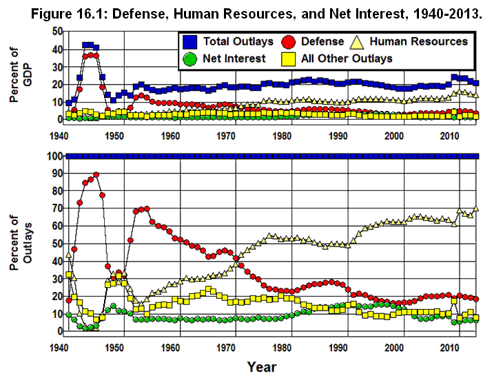
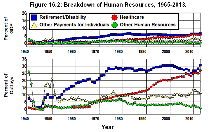
Where Did All The Money Go?
Chapter 17: Social Security, Healthcare, and Taxes
George H. Blackford © 2012
The deficit in the federal budget was 9% of GDP in 2010, and on December 1 of that year we were told by Erskine Bowles and Alan Simpson, co-chairs of the President’s National Commission on Fiscal Responsibility and Reform, that there was a $5.4 trillion unfunded mandate in the Social Security system that must be dealt with.
The last time we were told something like this was back in 1983 when the federal deficit was 6.0% of GDP in the aftermath of the 1981-1982 recession, following the 1981 Reagan tax cuts, and at the beginning of Reagan's anti Soviet defense buildup. At that time, the Social Security trust funds were dwindling, and Social Security was in danger of running out of money. In the midst of that fiscal mess, President Reagan established the Greenspan Commission to reform Social Security.
The Greenspan Commission
In accordance with the recommendations of the Greenspan Commission, Congress agreed to
Increase the payroll taxes paid by self employed individuals.
Increase the retirement age from 65 to 67 by 2022.
Accelerate previously scheduled payroll tax increases.
Require that 50% of the Social Security benefits received by higher income beneficiaries be taxed and paid into the Social Security trust fund.
Expand Social Security coverage to nonprofit and newly hired federal employees.
Congress also made a number of additional changes that, when combined with previously scheduled payroll tax and income cap increases, not only dealt with the trust fund problem, but changed Social Security from a pay-as-you-go system in which the money received by current beneficiaries is paid by current workers, to a partial-advanced-funding system in which the current workers prepaid a portion of their own retirement, Medicare, disability, and death benefits as they also paid for the benefits of the current beneficiaries. (SSA) As a result, Social Security has had an annual surplus since 1984—a surplus that increased the Social Security Old-Age Survivors and Disability Insurance (OASDI) trust fund to $2.6 trillion by 2011 with an additional $0.3 trillion in the Medicare and supplementary medical insurance trust funds as well.
Investing the Social Security Trust Fund
This $2.9 trillion represents the prepayment of the current working generations for their own retirement, medical, disability, and death benefits—payments they made into these trust funds while they fully supported (paid for) the retirement, medical, disability, and death benefits of the generations that went before. And what happened to this $2.9 trillion? It was placed in the safest investment on Earth: United States government bonds backed by the full faith and credit of the United States of America. Why? Not only because this is the safest investment on Earth, but because there was no acceptable alternative way to invest these funds.
If the Social Security Administration were to invest in non-government securities, it would involve the federal government in the private securities markets in a massive way. The potential for corruption with so much money involved was daunting, so much so that virtually no one thought this was a good idea. At the same time, the idea that these funds be divided into private accounts and invested in private securities by private individuals was also deemed unacceptable. This would make them vulnerable to the vagaries of the private-securities markets, and, as such, would defeat the central purpose of the Social Security System.
Social Security was created to provide a system of government guaranteed social insurance that is not dependent on the private-securities markets. It was the lack of such a system following the financial disaster in 1929 that inspired the Social Security System in the first place. What's more, the idea that the trust funds should have been invested in private securities was put to the test in the 2000s. It is only because these funds were invested in government bonds that they survived the stock market crash of the early 2000s and the financial crisis of 2008.
The Baby Boomer Problem
The baby boomer retirement problem is explained in The 2011 Annual Report of the Board of Trustees of the Federal Old-Age and Survivors Insurance and Federal Disability Insurance Trust Funds. A concise statement of this problem can be found in the Trustees' message to the public in the summary of this report:
Social Security expenditures exceeded the program’s non-interest income in 2010 for the first time since 1983. . . . This deficit is expected to shrink to about $20 billion for years 2012-2014 as the economy strengthens. After 2014, cash deficits are expected to grow rapidly as the number of beneficiaries continues to grow at a substantially faster rate than the number of covered workers. Through 2022 . . . redemptions will be less than interest earnings, [and] trust fund balances will continue to grow. After 2022, trust fund assets will be redeemed in amounts that exceed interest earnings until trust fund reserves are exhausted in 2036 . . . . Thereafter, tax income would be sufficient to pay only about three-quarters of scheduled benefits through 2085. (SSA)
The Trustees further explain in this message that
Program costs equaled roughly 4.2 percent of GDP in 2007, and are projected to increase gradually to 6.2 percent of GDP in 2035 and then decline to about 6.0 percent of GDP by 2050 and remain at about that level. (SSA)
This is what all of the fuss is about:
If we do nothing, the current payroll tax structure and trust fund is expected to carry the system into 2036 at which point the trust fund will be exhausted and payroll taxes will cover only 75% of the promised benefits. At that point either taxes will have to be raised or benefits cut to make up the difference.
The annual costs of Social Security benefits were 4.2% of GDP in 2007 and are expected to increase to 6.2% in 2035, then decline to 6.0% by 2050 and thereafter. This means that in order to maintain benefits, the proportion of GDP devoted to Social Security benefits must increase by 2.0% of GDP (6.2-4.2=2.0) between 2007 and 2035 and decrease thereafter by 0.2% of GDP between 2035 and 2050 for a net increase of 1.8% of GDP from 2007 through 2050.
Where's the crisis? According to the Trustee’s report, the Social Security trust fund is expected to continue to increase until 2022, and Social Security is fully funded until 2036. Social Security benefits must increase by 2% of GDP by 2035, which would not seem like much of a problem since the United Sates is one of the wealthiest countries on Earth. Increasing Social Security benefits by 2% of GDP between now and 2035 should not be a major problem.
What's more, the trustees assume in their report that over the next 75 years productivity, as measured by output produced per hour of labor, will increase in the United States at an annual rate of 1.7%. This is the average rate of productivity growth for the past forty years, and if productivity continues to grow at this rate it means, through the magic of compounding, our economy will be 50% (1.017 multiplied by itself 25 times = 1.52) more productive in 2035 than it was in 2010. Even if productivity only grows by the worst case scenario considered in the trustees’ report, 1.3% a year, we will still be almost 40% (1.013 multiplied by itself 25 times = 1.38) more productive in 2035. Why should we believe that an increase of Social Security benefits equal to 2% of GDP between now and 2035 is going to be a crushing burden on society in a world in which the labor force that produces that GDP will be able to produce 40% to 50% more per hour of work than we do today? (Baker)
It's time to step back, take a deep breath, and remember what we are talking about here. We are talking about increasing the share of GDP that is devoted to the payment of Social Security benefits from 4.2% today to 6.2% by 2035, then a decline in this share to 6.0% by 2050. This is a net increase of only 2.0% of GDP over the next twenty-five years. At the same time, productivity is supposed to increase 40% to 50% by 2035. This is the economic problem posed by the baby boomers' retirement, a problem that most certainly must be dealt with, but it is not a problem that portends a budget crisis that will require drastic changes in the Social Security System to solve.
Figure 17.1, which plots federal expenditures as a percent of GDP from 1965 through 2012, should help to put this problem in perspective.
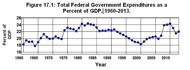
Source: Source: Office of Management and Budget. (1.2)
As is indicated in this figure, the average of federal expenditure as a percent of GDP during the 1980s (22.2%) was 2 percentage points above the average in the 2000s (20.3%). In other words, an increase in Social Security benefits equal to 2% of GDP by 2035 would be the equivalent of taking us back to where we were in the 1980s in terms of the federal budget. This would hardly require a dramatic change in the American way of life, especially since productivity today is 40% to 50% greater than it was in the 1980s and is expected to be 40% to 50% greater in 2035 than it is today. What’s the big deal about the baby boomers increasing Social Security payments by 2% of GDP between 2010 and 2035 in a world in which output, and, hence, real income per worker is expected to be 40% to 50% greater than it is today?
Legacy of the Greenspan Commission
It is essential to recognize, however, that even though the existence of a $2.6 trillion trust fund goes a long way toward solving the funding problem the baby boomers present to the Social Security Administration, it adds nothing toward solving the fiscal problem faced by the federal government. The reason is that the Greenspan Commission’s partial-advanced-funding scheme does not change the fiscal situation of the government when it comes time for the baby boomers to retire.
As we saw in Chapter 11, back in the 1980s, the Reagan Tax Cuts led to huge deficits in the federal budget that were not brought under control until the 1990s. One of the mechanisms that helped to bring these deficits under control was the increase payroll taxes paid by working people as the Social Security System was converted from a pay-as-you-go system to a partial-advanced-funding system. As was noted above, since the mid 1980s Social Security has had an annual surplus, a surplus that increased the Social Security OASDI trust fund by $2.6 trillion. These funds were, in turn, lent to the federal government to help finance its general expenditures, to the effect that by 2001 the money borrowed from the Social Security System’s trust funds in that year alone amounted to 8.75% of the federal budget.
The problem is, as the baby boomers began to retire in the early 2000s, the amount of cash available to be borrowed from the Social Security System began to dwindle, and in 2010 there was no cash left to borrow even though the Social Security System still had a surplus in that year. The reason is that even though there was a surplus in the budget for Social Security in that year, the amount of cash the system took in from payroll taxes was less than the amount of cash it paid out in benefits and costs. This situation is explained in the passage from the Trustee's Report quoted above:
Social Security expenditures exceeded the program’s non-interest income in 2010 for the first time since 1983. . . .Through 2022 . . . redemptions will be less than interest earnings, [and the] trust fund balances will continue to grow. After 2022, trust fund assets will be redeemed in amounts that exceed interest earnings. . . (TRSUM)
This means that in 2010 the government could no longer simply credit the interest it owed the Social Security System to its account and borrow its surplus cash since there was no surplus cash left to borrow. There was a cash deficit in the Social Security systems accounts, and the federal government was forced to pay a portion of the interest it owed the system in cash in order to fund this cash deficit.
As a result, since 2010 the federal government has been forced to pay a portion of its interest obligation to the Social Security System in cash in order for the Social Security System to pay its benefits and administrative costs in cash. At the same time, the amount of money the federal government owes the Social Security trust funds each year continues to grow because the amount of cash the federal government has been forced to pay into the Social Security System each year has been less than the amount of interest that accrues each year on the debt the federal government owes to the system. The difference must be credited to the Social Security System's trust fund which, in turn, increases the trust fund.
This situation is expected to continue through 2022 when the Social Security System's cash deficit is expected to equal the amount of interest the government owes the system in that year. At that point the Social Security trust fund is expected to peak, and from then on the trust fund is expected to fall as the federal government is forced to redeem the government bonds in the Social Security trust fund (as well as pay the interest that accrues each year on its remaining debt to the Social Security trust fund) in cash in order for the Social Security System to meet its obligation to pay its administrative costs and benefit payments to the baby boomers in cash.
There are only two ways the federal government can come up with the cash needed to pay the interest on its debt to the Social Security System and to begin paying back the principal it borrowed from working people: It can either raise taxes or borrow the needed funds. If it doesn’t raise taxes, it will have to borrow, and it can’t borrow without increasing the national debt. The only alternative is for the federal government to default on its obligations to the baby boomers by reducing their Social Security benefits.
Thus, when it comes to making up the difference between payroll tax receipts taken in and benefits paid out it makes no difference whether there is a trust fund or not. In either case, the government must either borrow or tax to make up this difference. As a result, the trust fund has no effect on the fiscal situation facing the government when the benefits owed the baby boomers come due.[17.1]
But if prepaying a portion of their Social Security benefits did not contribute to a solution to the government's fiscal problem when the baby boom generation retires, just what did the Greenspan Commission accomplished? What it accomplished was an increase in the taxes paid by working people to support the general expenditures of the government. That increase yielded the government $2.9 trillion from working people since 1983 that it would not have received if the Social Security System had stayed on a pay-as-you-go basis. That's what prepaying a portion of the Social Security benefits accomplished, and that's all it accomplished from the perspective of the fiscal soundness of the government.
This is where the real crisis in Social Security lies, and this is not an economic crisis. We are still talking about increasing Social Security benefits by only 2% of GDP by 2035 in a situation where increases in productivity is expected to increase output per worker by 40% or 50%. It is a moral and political crisis, however, because our society has to decide how it is going to come up with the funds necessary to make this adjustment or if it is going to not come up with these funds and renege on its promise to the baby boomers. (Surowiecki)
The Moment of Truth Report
The bipartisan Moment of Truth report written by Alan Simpson and Erskine Bowles is the end product of the President’s National Commission on Fiscal Responsibility and Reform. While this report was formally rejected by the Commission, it puts forth a set of recommendations to deal with our federal deficit and debt problems in a comprehensive way, recommendations that have gained a significant amount of political support. Of particular interest in this report are the recommendations regarding Social Security, Medicare, and revisions of the tax code.
Social Security
Concerning Social Security, the Simpson-Bowles recommendations are summarized in Figure 17.2.
Source: Moment of Truth Report.
These recommendations contain five key elements:
Gradually phase in progressive changes to the benefit formula while increasing the minimum benefit and adding a longevity benefit. (29%)
Index retirement age and earliest eligibility age to increase with longevity. (18%)
Use a chained CPI rather than the standard CPI to adjust benefits for changes in the cost of living. (26%)
Gradually increase the income cap to cover 90% of wage income. (35%)
Add newly hired state and local government employees to the program after 2020. (8%)
The percentage in parentheses following each item indicates its contribution toward eliminating the expected shortfall in Social Security funding over the next seventy-five years.
The first element in this list combines the first, second, and forth items in Figure 17.4 where the savings are supposed to be achieved by making the benefit payout system more progressive—that is, by lowering the benefits paid to high income recipients while, at the same time, increasing the benefits paid to low income recipients. The suggestion that these savings are coming from making the system more progressive is rather disingenuous, however, in that the savings come from a net cut in benefits, not from the fact that the resulting payout scheme is more progressive. If the increase in benefits paid to low wage earners were equal to the decrease in benefits paid to higher wage earners there would be no savings from this adjustment in progressivity.
The second item obviously achieves the savings, without any pretext, through a straightforward across the board cut in benefits by increasing the retirement age. The third also achieves the savings by cutting benefits by way of a controversial change in the way the Social Security cost of living adjustment is calculated. (WSJ SGS) The last two achieve their savings by increasing the payroll tax base.
Thus, when we do the math, we find that these recommendations solve Social Security’s future revenue problem by cutting benefits to cover 73% of the expected shortfall and by expanding the tax base to cover an additional 43% of the shortfall. (Presumably, the redundant 16% of savings is there to maintain the Social Security trust fund that will be lent to the government.) According to Simpson and Bowles, if we accept their recommendations Social Security will be on a sound financial footing for the next 75 years.
It is worth noting, however, that if these recommendations are implemented they will have the effect of converting Social Security from an insurance program in which the benefits provide some protection against a catastrophic loss into a kind of non-means-tested welfare program for the elderly in which there are hardly any benefits at all. The extent to which this is so is indicated in Figure 17.3 which shows the expected payout under the current law and how the payout structure would change under the Simpson-Bowles recommendations.
Source: www.StrengthenSocialSecurity.org, Benefits Chart.
Under this scheme benefits would fall by 47% for "'Maximum' Earners($106,800)", 39% for "'High' Earners ($68,934)", 27% for "'Medium' Earners ($43,084)" and even "'Low Earners' ($19,388)" would see a decrease. In addition, only 40% of the "'Very Low Earners' ($10,771)" would see an increase while the remaining 60% would see their benefits fall. This is not Social Security as we know it.
Even worse, the Simpson-Bowles scheme proposes to fund this program through the payroll tax. The payroll tax is one of the most regressive taxes there is. It is levied only on earned income (income received from wages and salaries) with no deductions and only minor exemptions, and the total amount of earned income taxed is capped where the cap in 2011 was $106,800. It is not levied on unearned income (income received in the form of interest, dividends, capital gains, rent, and corporate profits) or on earned income above the $106,800 cap. As a result, virtually all of the income of low income families is subject to the Social Security tax since virtually all of their income comes from wages and salaries below the cap, while virtually none of the income of the wealthy is subject to this tax since virtually all of their income is either above the cap on earned income or comes from unearned income.
The payroll tax is hardly an equitable way to finance a welfare type program. The burden of financing this sort of program should fall heaviest on those who can afford to pay, not on the backs of the working poor as is the case when the payroll tax is used. It makes sense to use a payroll tax to finance an insurance program. It does not make sense to use a payroll tax to finance a welfare-type program.
Healthcare
Our multiple-payer, third-party, fee-for-service payment healthcare system whereby healthcare providers decide with patients what services to provide and how much to charge while insurance companies or the government picks up the tab virtually guarantees continually increasing costs. There is a powerful incentive to over prescribe in this system and little incentive to deliver quality healthcare in a cost effective manner since the decisions as to what to charge and how much to prescribe are made primarily by providers.
To make matters worse, rising healthcare costs virtually guarantee that a continually increasing share of the healthcare costs will be passed on to the government as the higher costs force people, especially those with poor health, out of the private healthcare system. This is so because as people are forced out of the system society must decide the extent to which the government should pick up the tab for those who can no longer afford the cost of private healthcare. To the extent the government picks up the tab, it reinforces the process of third-party payment irrespective of cost that leads to the increasing costs that forces people out of the private healthcare system in the first place. To the extent the government does not pick up the tab, people who could otherwise be saved are left to die or to suffer with maladies that could otherwise be cured. This choice begs the question: How many poor people who cannot afford to pay for the cost of healthcare should be allowed to suffer or die—in the wealthiest country on Earth—in order to lower the costs for those who can afford to pay?
There is no optimal answer to this question that is in any sense humane, and our attempt to find one over the past 75 years while at the same time attempting to hang on to our archaic multiple-payer, third-party, fee-for-service payment system has caused the American healthcare system to become the least efficient among the advanced countries of the world. We rank 51th in terms of life expectancy, 51th in terms of infant mortality, 24th in terms of the availability of doctors, 25th in terms of mother’s health, 37th in terms of the overall performance of our healthcare system, and at the same time, we spend more for healthcare per person and as a percent of GDP than any other country in the world. (OECD OECD Charts NYT IOM JAMA1 JAMA2)
Over the past thirty years healthcare expenditures as a percent of GDP have increased at the rate of 2.2% per year. At this rate, expenditures as percent of GDP will double every 32 years. Obviously something is going to give before this can occurred. The only question is what: the government’s budget, employer sponsored health insurance, or both?
The Patient Protection and Affordable Care Act has attempted to address this rising healthcare cost problem, but while there are a number of cost saving provisions in this bill, the Affordable Care Act hangs on to the fee-for-service, multi-third-party-payer model. There is no single-payer mechanism or public-option plan provided for in this act to provide a direct mechanism by which costs can be controlled. In addition, the 85% payout restriction on insurance companies that is part of this bill means that once insurance companies reach this limit they will only be able to increase their profits in the aggregate if healthcare costs increase, thereby, increasing what insurance companies can make from their 15% cut. This does not exactly provide an incentive for insurance companies or providers to hold down costs, and if healthcare costs continue to grow the way they have in the past, the cost of Medicare and Medicaid, which together make up the largest single component of our social insurance system today, will eventually become unbearable.
In dealing with healthcare, the main thrust of the Simpson’s-Bowles recommendations is to reduce healthcare costs by forcing healthcare recipients, both public and private, to pay a larger proportion of the cost. But, as was noted above, this plan can only reduce costs to the extent it forces those who cannot afford the added costs out of the healthcare system with all of the implications that has for the health of our population; to the extent the government picks up the tab for those who cannot afford the added cost there is no saving. This plan is just more of the same kind of thing we have been doing for the past 65 years, and there is no reason to think the results will be different: rising healthcare costs with a larger and larger portion of the tab being picked up by the government.
Reforming the Tax Code
What is particularly disturbing about the Simpson-Bowles bipartisan plan for deficit reduction, however, is that while they recommend massive cuts in Social Security and Medicare benefits, at the same time they recommend the top marginal income tax rate paid by corporations and the wealthy be cut from 35% to 28%, that the marginal income tax rate paid by middle-income earners be set at 22%, and that the lowest income tax rate paid by the not so wealthy be increased from 10% to 12%.
It these changes are passed into law, the combined 14.2% [17.2] employee/employer payroll tax rate plus the income tax rate in the lowest income bracket will equal 26.3%—less than two percentage points below the maximum marginal rate corporations and multibillionaires will pay. Those in lower end of the middle tax bracket will face a combined marginal rate of 36.2%—8.2 percentage points above the marginal rate multibillionaires and corporations will pay. Even though Simpson and Bowles also recommend treating dividends and capital gains as ordinary income and recommend a few other changes that will make the tax code somewhat more progressive, there is something very wrong here.
There was a surplus in the federal budget equal to 2.4% of GDP in 2000 before the massive 2001-2003 Bush tax cuts, before the invasion of Iraq, and before those who ran our financial institutions devastated our economy. The fiscal problems we face today are clearly the result of the Bush cut taxes combined with the increases in defense expenditures squandered in Iraq and the devastating recession brought on by the fraudulent, reckless, and irresponsible behavior of those in charge of our financial institutions. Social Security and Medicare had nothing to do with this mess.
And yet—in the name of fiscal responsibility—Alan Simpson and Erskine Bowles, acting as co-chairs of the National Commission on Fiscal Responsibility and Reform, released their Moment of Truth report in which they propose we 1) cut Medicare benefits and increase the private cost of healthcare dramatically, 2) convert Social Security into a welfare-type program paid for with payroll taxes in order to avoid paying an increase in benefits equal to 2% of GDP, and, at the same time, 3) give additional tax cuts to those at the top of the income distribution, many of whom made fortunes out of the Iraq war and through financing the housing bubble that devastated the economy of the entire world. And to add insult to injury, we are also supposed to increase the taxes paid by those in the lowest income tax bracket. This not only defies common sense, it defies common decency.
An Alternative Approach
The Moment of Truth report released by the co-chairs of the National Commission on Fiscal Responsibility and Reform does not deal with the deficit problem in a substantive way. There is no discussion as to how the optimum level or quality healthcare can be provided to the population in the most cost effective manner in their report. No discussion as to how Social Security and Medicare can be maintained as viable insurance programs. No discussion as to how the optimum level of essential government services can be made available in their most cost effective manner.
This report concentrates only on cutting government services and lowering tax rates paid by the ultra wealthy. As a result, it simply ignores obvious solutions to our Social Security, healthcare, and fiscal problems—solutions that do not entail emasculating Social Security and Medicare.
Social Security
There are many ways to deal with the expected shortfall in Social Security revenues needed to finance the benefits promised to the baby boomers that would not involve drastic changes in the Social Security program. One would be to
Increase the payroll cap to apply to 90% of covered earnings as Congress intended back in 1977 or, perhaps, to an even higher percentage.
Convert the federal estate tax to a dedicated Social Security tax that is credited automatically to the Social Security trust fund.
Expand the program to cover newly hired state and local workers.
Implement modest changes in payroll taxes and Social Security benefits, if needed, after the above changes have been made and, perhaps, extend the payroll tax to include unearned income and/or remove the income cap altogether.
Approaching the expected Social Security deficit problem in this way would not require the draconian cuts in benefits put forth in the Moment of Truth Report nor would it require draconian payroll tax increases.
Healthcare
As we saw in Chapter 12, through Chapter 16, it is the rising cost of healthcare that poses the most serious fiscal problem faced by the federal government, and, as has been noted above, every advanced country in the world that has better health statistics and lower healthcare costs than we do has abandoned the cost ineffective multiple-third-party payment system for a single-payer universal healthcare system that provides government subsidized healthcare for all—paid for through taxes—where costs are controlled through government negotiated prices. They pay higher taxes than we do, but their higher taxes are more than offset by the savings in insurance premiums and lower healthcare costs—not to mention the fact that they are healthier than we are, and they live longer than we do. (OECD OECD Charts NYT IOM JAMA1 JAMA2)
The simplest, most efficient, and most cost effective way to provide a comparable system for the United States would be to extend the Medicare program to the entire population. This program works, and the institutions necessary to run it are already in place. It would take very little effort to retool Medicare to meet the needs of the entire population compared to the massive effort it is going to take to implement the Patient Protection and Affordable Care Act.
Reforming the Tax Code
By 2000, increases in the Social Security trust fund was adding over $150 billion a year in cash flow and deferred interest payments to the government’s general fund, and it continued to do so for the next eight years. From 1996 through 2008, the federal government relied on the increase in the OASDI trust fund to finance over 6% of its outlays and, as was noted above, this reached a peak in 2001when the money borrowed from the Social Security System’s trust funds in that year alone amounted to 8.75% of the federal budget.
Now that the baby boomers are starting to retire, this source of revenue is coming to an end. While some of the interest the government owes the Social Security System each year can still be simply added to the System's trust funds, cash receipts from payroll taxes have fallen below the cash benefits and administrative costs the Social Security System must pay out. As a result, the government must either borrow the difference or it must increase non-payroll taxes in order to pay that portion of the interest it owes the Social Security System each year in cash to meet this cash shortfall—if that’s what our government chooses to do. It also has the option of reneging on its agreement with the baby boomers by reducing their benefits or increasing the payroll taxes paid by their children and grandchildren.
Even though there are a number of simple fixes that will solve the Social Security baby boomer retirement problem, and it would be fairly easy to fix our healthcare system, none of these fixes will work if the federal government is not made fiscally sound. These fixes can only work if we come up with the funds needed to make them work while, at the same time, coming up with the funds needed to provide the other government services the American people demand.
As we saw in Chapter 16, what this means is that, if we are to preserve Social Security, Medicare, and provide for all of the other government services that are demanded by the American people, we must raise taxes. (Fieldhouse Diamond Sides)
Reregulating the Financial System
It will, of course, also be necessary to reregulate our financial system if we are to keep our financial institutions from creating the kinds of economic disasters that unregulated financial institutions have created throughout history. At the very lease we must
Glass-Steagall Act to eliminate the kinds conflicts of interests inherent in conglomerate mega-bank financial institutions,
reenact the
break up those financial institutions that are "too big to fail," and
provide for direct regulation of hedge funds, over-the-counter derivatives, and the market for repurchase agreements with the power to set margin requirements for repurchase agreement loans and capital requirements for Credit Default Swaps.
These are the minimum actions required to keep those in charge of our financial institutions from creating in the future the kind of economic catastrophes they have created in the past when unrestrained by government regulation—the kind of economic catastrophe we are in the midst of today.
Simply passing laws, however, is not enough. Government regulation begins with the law, but it ends with the regulators. It was the belief in free-market ideology that was the primary cause of the financial crisis we face today, not the absence of legislation. The Home Ownership and Equity Protection Act (HOEPA) passed 1994 gave the Federal Reserve the absolute authority to regulate the mortgage market. Enforcing the laws against predatory lending practices, enforcing strict underwriting standards for mortgage loans, and setting maximum loan to value ratios on mortgages would have prevented the housing bubble that came into being in the 2000s. The Federal Reserve had the absolute authority to do all of these things under HOEPA during the housing bubble, but the ideological faith in free markets to regulate themselves on the part of regulators, the administrations, and the Congress kept the Fed from doing so. (Bair)
In addition, the regulators could have petitioned the government to bring Money Market Mutual Funds, Cash Management Accounts, and repurchase agreements under the purview of depository regulators during the Reagan administration and to extend the regulatory authority of the Security and Exchange Commission and Commodity Futures Trading Commission to regulate hedge funds and the markets for Credit Default Swaps during the Clinton administration, but, again, ideology stood in the way.
Until the terribly misguided view of reality embodied in the failed nineteenth-century ideology of free-market capitalism is replaced in the minds regulators, administrations, Congress, and the body politic by a pragmatic view of financial regulation that recognizes the need for the government to rein in and control the speculative and fraudulent urges of the financial sector there is little hope of our being able to survive the current crisis with our basic social institutions intact or to avoid similar economic catastrophes in the future.
Reviving the Economy
As was noted at the end of Chapter 3, today we are faced with the same kind of situation we faced in the 1930s: Given the state of mass-production technology, the distribution of income is incapable of providing the domestic mass markets needed to achieve full employment in the absence of a speculative bubble. If we do not come to grips with this problem our domestic markets for mass-produced goods will continue to erode; we will be plagued with boom and bust cycles of economic instability, and it will be impossible to maintain the standard of living of the vast majority of our population as our economic resources are transferred out of those industries that produce for domestic mass markets and into those industries that produce for the privileged few. (King)
Not only will it be impossible to maintain the standard of living of the vast majority of our population if the concentration of income is not reduced, those at the top of the income distribution will eventually find they are getting a larger piece of an ever decreasing pie. It is domestic mass markets that make mass production possible, and it is mass production—made possible by our domestic mass markets—that made the United States the economic powerhouse of the world. The erosion of our domestic mass markets erodes the very foundation on which our economic system rests, and to the extent that foundation is undermined, our ability to produce is undermined as well. (Ostry)
The only way a country can take advantage of mass-production technologies in the absence of an income distribution that provides a domestic mass market capable of purchasing output produced without increasing debt relative to income is by producing for export and running a current account surplus. Unfortunately, continually running a current account surplus leads to increasing the debts of foreigners relative to their incomes, especially when those debts are accumulated through the process of financing consumption or the production of capital goods in the midst of speculative bubbles that do not increase productivity. Increasing domestic debt relative to income, or the debts of foreigners relative to their incomes is not sustainable in the long run. The transfer burden from debtor to creditor must eventually overwhelm the system, and must eventually lead to a financial crisis that causes the system to collapse.
In the final analysis, it was the rising debts in the importing countries relative to their incomes that led to the current crisis. The only way to avoid this kind of crisis is through producing for domestic markets without a continually increasing debt relative to income. This, in turn, requires a distribution of income capable of supporting the domestic mass markets needed to purchase the domestic output that can be produced.
Given the extent to which non-federal debt has increased relative to income over the past twenty-five years it should be obvious that we are not going to be able to solve the economic problems we face today without a major intervention on the part of the federal government. Simply raising taxes is not going to solve our deficit/debt problem or return our economy to full employment. As we saw in Chapter 3 and again in Chapter 15, it was the massive government expenditures during World War II that finally brought us out of the Great Depression, and it was the fall in concentration of income during and following the war that made it possible for our mass production industries to survive. There is no reason to believe we will be able to survive the current crisis with our basic social institutions intact and without a fall in the standard of living of the vast majority of the population in the absence of a similar effort on the part of the federal government today and without a similar reduction in the concentration of income.
The government has already had to step in to the tune of $700 billion in TARP funds and trillions of dollars of guarantees in order to bail out the financial institutions that brought the current crisis down upon us, but this is only placing a band aid on the economic wound we suffered as this bailout transferred wealth and income from taxpayers to the bankers who caused the problem in the first place. It is the mortgagors that should have been bailed out, not the bankers who created the problems we face today. (Bair) The fiscal resources of the federal government should be used to increase taxes and government expenditures to mitigate the effects of the current recession and rebuild the public infrastructure we have allowed to deteriorate over the past thirty years. They should not be squandered on lower taxes for corporations and the higher income brackets or on bailing out those who created the financial house of cards that has fallen down upon us.
Mobilizing our fiscal recourses by increasing taxes and government expenditures to provide relief to those whose mortgages are underwater and waging a war on our deteriorating public infrastructure certainly makes more sense than waiting for—or manufacturing—a real war to justify the mobilization of these resources. If we do not approach our non-federal debt and unemployment problems by increasing taxes and government expenditures in a way that makes it possible to deleverage the system while improving our public infrastructure our economic situation can only get worse as our financial system struggles to survive. Our unemployment problem will persist, and eventually the productivity of our economic resources will begin to fall as our economic resources are transferred out of those industries that produce for domestic mass markets. Our transportation, water and waste treatment facilities, education, power distribution, communication, regulatory, legal, and other governmental systems will continue to deteriorate, and it will be impossible to maintain the standard of living of the vast majority of our population.
These things should be obvious, and, yet, our political leaders (at home and those in Europe as well) are in the process of negotiating how best to cut government expenditures and “entitlement” programs—the very expenditures that kept our economy from spiraling in to the abyss it spiraled into in the 1930s and the very programs that allowed us to avoid the wretched squalor and misery we experienced during that dismal period of our history—and, at the same time, they are negotiating how best to lower taxes on the upper income groups even further.
At the center of these negations is the Moment of Truth Report written by Alan Simpson and Erskine Bowles—the end product of the President’s National Commission on Fiscal Responsibility and Reform. As we saw above, the primary recommendations of this report are to
Convert Social Security from an insurance program in which the vast majority of the participants benefit, into a non-means-tested welfare program for the elderly, funded by a regressive payroll tax, in which only the poorest of the poor benefit.
Reduce healthcare costs by forcing healthcare recipients, both public and private, to pay a larger proportion of the cost directly thereby forcing those who cannot afford the added costs out of the healthcare system—the ultimate death panel solution to the healthcare cost problem whereby those who can’t afford the added costs are simply allowed to suffer and die.
Cut the maximum marginal tax rate paid by corporations and multibillionaires from 35% to 28%, set the middle tax bracket at 22%, and increase the tax rate paid by the lowest income earners from 10% to 12% thereby creating a situation in which the combined 14.2% employee/employer payroll tax rate plus the income tax rate in the lowest income bracket will equal 26.2%—less than two percentage point below the 28% marginal rate corporations and multibillionaires will pay. Those toward the lower end of the middle bracket will face a combined marginal rate of 36.2%—8.2 percentage points above the marginal rate multibillionaires and corporations will pay.
At the same time, the Dodd-Frank Wall Street Reform and Consumer Protection Act has added restrictions on the Federal Reserve’s ability to act in an emergency situation, (Bair) and the fundamental provisions of this bill do not go near far enough to eliminate the conflicts of interest in our financial system or to reign in the behavior of our financial institutions. In addition, those provisions of this bill that do hold some promise to moderated the fraud and deception that has pervaded our financial system over the past thirty years, the Consumer Financial Protection Bureau for example, are under attack on ideological grounds by a large segment of the politically powerful.
The ultimate question is whether we are going to deal with our problems by increasing taxes and thereby enhance the government’s ability to solve them, or are we going to follow the mantra of the free-market ideologues and undermine the government’s ability to deal with these problems by cutting taxes and government expenditures, dismantling our social-insurance programs, turning Federal Reserve policy over to Congress and, thereby, cut the threads that have so far saved us from the fate of the 1930s.
Lower taxes, less government, and deregulation caused the economic problems we have today, and more of the same is not going to solve these problems. If we are to solve these problems we must strengthen government, not weaken it; we must increase taxes, not lower them, and we must increase government expenditures as we rebuild the regulatory systems that were dismantled since the 1970s and rebuild the public infrastructure that has been allowed to deteriorate over the past forty years.
If we do not do these things and, instead, continue to follow the failed ideological mantra of lower taxes, less government, and deregulation we are most certainly going to end up right back where we started in the 1930s. And if the political leaders throughout the world continue to follow this failed ideological mantra and refuse to come to grips with the root causes of the worldwide economic catastrophe we face today, we are likely to end up where we ended up in the 1940s.
Endnote
[17.1] It should be noted that privatizing individual Social Security accounts also does nothing to solve the baby boomer retirement problem. Even if the Social Security system were made up entirely of individualized accounts that contained the government bonds now in the trust fund these bonds would still have to be redeemed by the government when the owners of these accounts began withdrawing retirement funds, or some non-Social-Security-account buyer would have to be found who is willing to purchase these government bonds.
The situation would be even worse, not for the government but for the Social Security account holders, if the private accounts contained private securities. Aside from the vagaries of the private securities markets, the flow of funds into the private securities markets as the baby boomers built up their accounts would have undoubtedly been a boon to these markets. It is just as undoubtable that the flow of funds out of these markets as the baby boomers retired would be a serious drag on these markets. The baby boomers would be buying as they drove prices up and selling as they drove prices down, not exactly a formula for getting rich. Such a scheme would, perhaps, serve the older baby boomers well, but certainly not the younger baby boomers.
[17.2] The combined rate is 14.2% rather than 15.3% since in combining the rates paid by the employer and employee we must include the portion of the payroll tax paid by the employer as part of the employee's income.
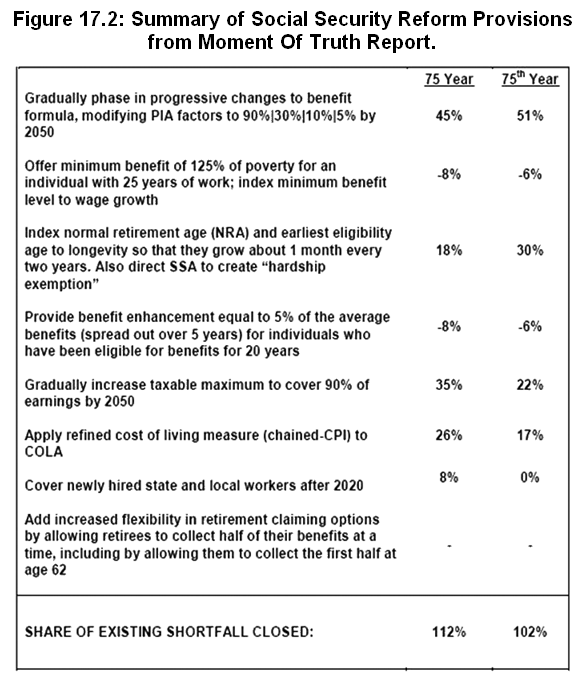
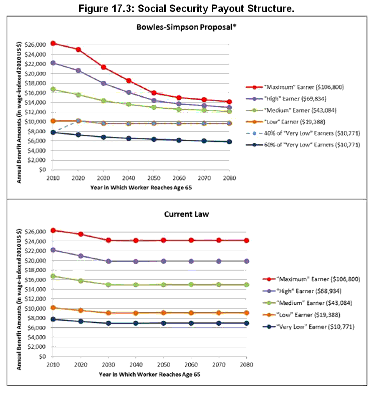
Where Did All The Money Go?
Chapter 18: Ideology Versus Reality
George H. Blackford © 5/16/2013
For the past forty years the Conservative Movement has incessantly attacked the American government as if the solution to all of our problems is to be found in lowering taxes, cutting government expenditures, and in getting rid of government regulations.
Few people seem to realize that this movement is attacking the same government that created the Social Security System to provide old age and disability insurance; Medicare, and Medicaid to provide health insurance for the aged and the indigent; the Veterans Administration to serve our veterans; unemployment compensation to soften the blow of unemployment for the unemployed; the Food and Drug Administration to protect us from tainted food and worthless or dangerous drugs; the Security Exchange Commission to fight fraud in the financial sector of our economy; the Federal Reserve System to control the money supply and provide for economic stability; the Consumer Protection Agency to protect us from dangerous consumer products; the Environmental Protection Agency to prevent the poisoning of the air we breathe, the water we drink, and the very ground on which we live; the Occupational Safety and Health Administration to provide for a safer workplace; the National Institute of Health to promote health research; the Centers for Communicable Desease and public health departments that fight the spread of communicable diseases; the National Science Foundation that promotes basic scientific research; and countless other institutions and regulatory agencies that promote the general Welfare, as is called for in the Constitution.
It is also the same government that created the transcontinental railroad and interstate highway systems along with all of our state highways, county roads, and city streets; the military that provides for our national defense; the police and judicial systems which set the rules and provide for law and order within society; our firefighters who fight our fires; our national, state, and local park systems; and our land-grant college system and other public college, university, secondary, and elementary school systems devoted to the concept of universal education that has proved to be the backbone of economic and social development within our society for the past 150 years. And this is the same government that won World War II and the Cold War and that has fueled the most powerful economic engine in the world.
These are all the products of our government, and it is this government conservatives have been attacking for the past forty years—the government of the United States of America as created by the Constitution of the United States of America. (Kuttner Lindert Amy)
Why We Regulate Markets
Contrary to what free-market ideologues would have you believe, there is a reason why we have government regulations. In the real world, government regulations are essential to the efficient and safe functioning of markets.
We regulate the markets for food and drugs and other consumer goods because without regulation it is inevitable that dangerous foods and drugs and consumer goods that have the potential to cause great harm to innocent people will be fraudulently or negligently foisted on an unsuspecting public.
We regulate markets to control pollution because without regulation it is inevitable that our air and water, rivers and streams, fish and fowl, and even the very Earth on which we live will become contaminated and poisonous to human beings.
We regulate the work environment because without regulation it is inevitable that the forces of competition and the drive for profit will lead to increasingly dangerous and harmful work environments with sixteen to eighteen hour days and eight and ten year old children working in coal mines.
Finally, we regulate financial markets not only because without regulation it is inevitable that greed and the lust for profit will lead to fraudulent, reckless, irresponsible, and foolish behavior on the part of those in charge of our financial institutions that will cause a great deal of harm, not only to the individual victims who are directly affected by this kind of behavior, but because throughout history, time and time again, we find that this kind of fraudulent, reckless, irresponsible, and foolish behavior has led to economic catastrophes that have brought the entire economic system to its knees—catastrophes that have led to an unconscionable amount of hardship, misery, and suffering on the part of innumerable individuals who had nothing to do with the nefarious behavior that brought on these catastrophes.
It is the presence of government regulation that moderates the forces within a capitalist system that, if left unchecked, would lead to injury and harm to a great number of innocent people, and it is the height of foolishness to think that somehow life would be better for the vast majority of the population if we did away with government regulation. The fact is, that in the absence of a powerful force to intervene in free markets to constrain them to serve humane ends, Capitalism promises to become a cancerous growth on humanity that will devour the very planet on which we live. The only force available to intervene in in this way is a democratic government, and it is clear from the history of Capitalism—or at least it should be clear—that we deny this reality at our peril. (Smith MacKay George Marx Veblen Roosevelt Haywood Jones Fisher Josephson Keynes Polanyi Schumpeter Boyer Galbraith Musgrave Domhoff Kindleberger Minsky
Skidelsky Stewart Zinn Stiglitz Phillips Kuttner Morris Taleb Lindert Bogle Harvey Dowd Galbraith Baker Stiglitz Klein Reinhart Fox Johnson Amy Sachs Smith Eichengreen Rodrik Graeber IPCC)We have been cutting back on government programs for forty years now, and it hasn't exactly worked out for the best as we continue to struggle with the end result of these cutbacks, namely, the worst economic crisis since the Great Depression and a governmental system that can barely function today.
Free-Market Ideology
The free-market ideologues that inspire the Conservative Movement have a very simplistic view of reality based on their concept of liberty and freedom. It is their belief that individuals should be allowed the freedom to fend for themselves in free and unfettered markets to provide for their own economic well being without government interference or guarantees. It is the free choices of individuals in free markets that create prosperity and wealth in society, in their view, and individuals owe nothing to society save to honor the contracts they freely enter into. And they definitely do not believe in government mandated social insurance. Government mandated social insurance interferes with the liberty and freedom of those, such as themselves, who do not wish participate in or pay for these programs. They simply do not believe that it is the purpose of government to promote the general Welfare, other than to provide for national defense and to protect property rights. (Friedman)
The leadership of the Conservative Movement also believes that if government will just get out of the way, the free choices of individuals in free and unfettered markets will optimize human well being within society through the discipline of the marketplace. Those who work hard and are productive will be rewarded by the marketplace through higher incomes and their ability to accumulate wealth in proportion to their contribution to society. Those who do not work hard, are not productive, and do not contribute substantially to society will not be so rewarded. (TP)
To the extent government interferes with this market discipline, people no longer have an incentive to work hard, productivity falters, output falls, and we are all made worse off. In this view, the distribution of income and wealth so determined by free and unregulated markets is fair and just, and anything the government attempts to do beyond national defense and enforcing property rights is unfair and unjust and does more harm than good as it destroys market discipline and causes productivity and output to fall.
The arguments explaining this view of reality are put forth with elegance and logical infallibility in such works as Ayn Rand's,The Fountainhead and Atlas Shrugged, Friedrich von Hayek's, The Road to Serfdom, Milton Friedman's, Capitalism and Freedom and Free to Choose, Ludwig von Mises’s, Human Action, and the American Conservative Union’s, Statement of Principles, works that have inspired conservatives to ever higher levels of passion over the past sixty years as well as having provided the backbone of their intellectual arguments.
In addition, the academic discipline of economics has provided a logically consistent and mathematically elegant model of market behavior that describes how this ideal system of human interaction in markets is supposed to work as well as the prerequisites for the existence for such a system to actually work. (Kuttner Taleb Dowd Galbraith Fox Musgrave Stiglitz Klein Johnson Smith)
It should not be surprising that the logically infallible works listed above combined with the heroic efforts of academic economists to explain how free markets are supposed to work have provided the intellectual foundation for an ideological view of society that is totally out of touch with reality. After all, you can prove anything with logic! All you have to do is start with a false premise, and the logically infallible works listed above are filled with false premises, beginning with the fact that the literature that provides the passion for this ideological view is based on a straw-man caricature of tyrannical government that completely ignores all of the essential functions that government performs in our daily lives and without which civilized society is impossible—the kinds of functions so beautifully explained by Douglas Amy in his website, www. governmentisgood. com.
By the same token, the academic model that explains how, and under what circumstances such an economy is supposed to work not only completely ignores the role of government in our economic and social lives, but the assumptions on which the logical consistency of this model depends—the most important being that no economic actor has the power to directly influence market prices, all market participants have perfect information as to the determination of market prices, that there are no external costs or benefits associated with the production or consumption of goods, and that people behave rationally—are impossible to achieve in the real world.
Income in the Real World
The free-market ideologues who dominate the Conservative Movement tell us that lower taxes, less government, and deregulated free markets will solve all of our economic problems and make everyone better off. Yet, when we look at the era at the beginning of the twentieth century in Figure 18.1 when taxes were low, government was small, and regulation was virtually nonexistent—a state of nature that conservative ideologues hold as ideal—we find that there was no increase at all in average real income of the bottom 90% of the income distribution. The real incomes of the bottom 90% didn't begin to increase during the twentieth centaury until 1933 at the beginning of the New Deal, that is, until the era of higher taxes, more government, and more regulation of the economic system ushered in by the New Deal began.
Source: The World Top Incomes Database.
What's more, when we look at the 40 year period that followed the beginning of the New Deal we find that the average real income of the bottom 90% (excluding capital gains) increase fivefold as it went from $6,940 (measured in 2012 prices) in 1933 to
$34,956 in 1973.We also find that during the 39 year period of lower taxes, less government, and deregulation that followed 1973 there was a repeat of the period that preceded 1933—no increase in the average real income of the bottom 90%. From 1974 through 2012, the average real income of the bottom 90% exceeded the high it had achieved in 1973 for only a brief, two-year period in 1999 and 2000, and by 2012 it had fallen back to $30,439, which was below the $31,205 level the bottom 90% had achieved in 1967.
In light of this history, the conservative's notion that
lower taxes, less government, and deregulation lead to prosperity for all is clearly absurd.Winners and Losers
It is obvious to all but free-market ideologues that the incomes people receive, and the wealth people are able to accumulate as they participate in a market economy, do not necessarily correspond to how hard they work or how productive they are or by how much they contribute to the society as a whole. It is also obvious that the accomplishments of individuals are not achieved by their own efforts alone, but are crucially dependent of the social system in which they live that makes their individual accomplishments possible.
No one can deny that the fortunes accumulated by Bill Gates, Paul Allen, Steve Jobs, Steve Wozniak, Robert Noyce, Gordon Moore, Andrew Grove, and countless others who have made immeasurable contributions to the micro computer revolution over the past forty years are comparable to their immeasurable contributions to the well being of the society as a whole and are well deserved on that account alone. They are living examples of everything the mythical world of unregulated, free-market capitalism is supposed to be about.
It is also true, however, that they did not achieve their immense accomplishments on their own. Their accomplishments were built on the backs of giants throughout history who developed the science that made their successes possible and depended crucially on the university system that has evolved over the centuries that made that science possible. Their successes would have been impossible without the tremendous technological breakthroughs in the aerospace program and as a result of government sponsored computer research during World War II, and there is a certain amount noncompetitive monopoly power that has contributed to the size of their fortunes.
At the same time, it is impossible to deny that luck played a major role in determining the size of their fortunes as well—that had they been born in a different era or into families living in desperate straits in Sub-Saharan Africa or some other desperate place in the world rather than in this era and into moderately well to do families in the United States they would have been far less successful in life. As a result of all of these social factors, and many more, they owe an immense debt of gratitude to the society that made it possible for them to flourish in the way they have flourished. (Alperovitz)
When we look at the income received and wealth accumulated by others in today’s world, however, we see a very different picture. When we look at the incomes received and fortunes accumulate by the executives of General Motors as they drove the world’s largest automobile company into bankruptcy; by the savings and loan owners and managers as they financed the commercial real estate bubbles in the 1980s; by the corporate raiders who drove American businesses deeper and deeper into debt and countless firms into bankruptcy; by those who hyped worthless internet stocks in the 1990s; by the executives of Drexel Burnham Lambert, Enron, Global Crossing, WorldCom, Fannie Mae, and countless other individuals that used insider information, stock manipulation, or phony accounting practices to generate paper profits to justify increases in their multimillion dollar salaries and bonuses as they ran the businesses they headed into the ground; by those who originated millions of subprime and alt-A mortgages through fraud and deception in the 2000s; and by those who gave unwarranted triple-A ratings to the mortgage backed securities, securitized these mortgages, and created the worldwide crisis we are in the midst of today we do not find living examples of everything the mythical world of unregulated, free-market capitalism is supposed to be about. Instead, we find living examples of what real-world, unregulated, free-market capitalism is actually about.
The unconscionable incomes and massive fortunes these individuals accumulated have nothing to do with economic efficiency or the contributions these individuals have made to the society as a whole. Their contributions to economic efficiency and to society as a whole were negative, and even if they returned all of the income they received and wealth they accumulated to the society that made their success possible there would still be a tremendous net loss.
Yet somehow, in the eyes of the free-market ideologue, the current economic catastrophe is supposed to be the fault of the individuals who lost their homes, their jobs, their life's savings, and their hopes and dreams for the future while those who perpetrated the fraud that caused this disaster and made billions of dollars in the process are not only held blameless but are, in fact, idolized by virtue of the fact that they made money on the deal. There is a terrible perversion in an ideological view of the world that blames the victims for allowing themselves to be preyed upon and extols the virtues of the predators who made fortunes in the process of creating a disaster for the rest of society.
The ideological explanation for the fall in real income for 90% of the families over the past forty years in terms of their refusal to work harder or because they haven’t increased their productivity or contributed more to the society as a whole makes no sense at all. Hours of overtime worked in the manufacturing sector increased by 67.9% from 1980 through 1995 while output per hour worked increased by at least 30% (and probably more than 50%), and total manufacturing output increased by 42.8%. At the same time, the average hourly earnings in the manufacturing sector decreased by 7.2% in real terms after adjusting for the increase in consumer prices. In other words, even though hourly workers in the manufacturing industries worked harder, were more productive, and the total output they produced to the benefit of the society as a whole increased, they were rewarded by a decrease in their real wage.
The incomes people receive and the wealth people are able to accumulate as they participate in a market economy depend as much on economic and political power as on hard work, productivity, and economic efficiency, and who has that power depends crucially on government policy. (Dillow) When government policy
opposes public financing of political campaigns and allows the money provided by political PACs, corporations, and wealthy individuals to dominate the political process,
favors unregulated markets,
allows the concentration of monopoly power into the hands of larger and larger corporations,
allows the profits of international banks and corporations to determine international trade and financial policy,
not only opposes collective bargaining on the part of labor unions, but employs government power to suppress strikes and refuses to enact and enforce laws against unfair labor practices,
provides massive subsidies to industry through the provision of public infrastructure, national defense, enforcement of civil law and order, and public education for the labor force as well as for the population at large, while at the same time
imposes a tax structure on the populace that does not recoup the costs of these subsidies from those who benefit from them the most, but, rather, places this burden on the backs of those who benefit from them the least
economic and political power gravitates into the hands of the economically and politically powerful few, and, as their incomes and wealth soar to astronomical heights, fraud and predation flourishes, the public infrastructure and social capital that made their success possible declines to the detriment of future generations, and the vast majority of the population founder in the wake of the economic catastrophes that result.
On the other hand, when government policy
provides public financing for political campaigns and offsets the money provided by political PACs, corporations, and wealthy individuals by providing equal time and equal funds to political campaigns,
favors regulating market behavior to promote the general Welfare,
prevents the concentration of monopoly power into the hands of larger and larger corporations whenever desirable and regulates the monopoly power that cannot be eliminated whenever necessary,
maintains a balance in trade that benefits the American people rather than maximizes the profits of international financial institutions and corporations,
not only encourages collective bargaining on the part of labor unions, but employs the power of government to enact and enforce laws against unfair labor practices,
provides massive subsidies to industry through the provision of public infrastructure, national defense, enforcement of civil law and order, and public education for the labor force as well as for the population at large while at the same time,
imposes a tax structure on the populace to recoup the costs of these massive subsidies from those who benefit from them the most and does not place this burden on the backs of those who benefit from them the least
economic and political power gravitates from the privileged few into the hands of the vast majority of the population, and, while the incomes and wealth of the few still grow to astronomical heights, the income and wealth of those few do not soar to such dizzying heights that the vast majority of the population is left behind. Income and wealth does not flow from the kinds of massive fraud and predation that lead to economic catastrophes, and the public infrastructure and social capital that made their success possible is able to grow to the benefit of future generations. (Amy Kuttner Musgrave Johnson Lakoff Galbraith Stewart Smith Black Rodrik Lindert Prasad Fieldhouse Diamond Sides)
Capitalism and Socialism
In the utopian world of free-market ideology it's all so simple: Deregulate the financial system; get rid of the EPA, SEC, FDA, CFTC, Social Security, Medicare, Medicaid, unemployment compensation; cut government expenditures; lower taxes, and all of our problems will go away. But in the real world it’s not that simple.
You do not have to be an economist to look around the world and see that unregulated, free-market capitalism is not the sine qua non of economic prosperity and social wellbeing. All of the most prosperous countries of the world, especially in North America and Western Europe, contain significant and essential elements of what right-wing ideologues call socialism. At the same time, the vast majority of people who live in non-socialist countries live in abject poverty. The fundamental difference between the prosperous and free, and the impoverished and enslaved throughout the world is the quality of their governments.
When you step back and look at the world as it actually is you find that all of the most productive economies in the world—in particular, those of Western Europe and North America—are what free-market ideologues call socialist countries; they all have a major portion of their economies dominated by government. Not only do they all have government provided public infrastructure (things like roads and highways, ports and airports, public health and sanitation, legal and criminal justice systems, and public education), they all have government provided social-insurance programs such as Social Security, government provided healthcare, unemployment compensation, and welfare assistance for the less fortunate.
The fact that all of these economic powerhouses have a substantial portion of the economies dominated by government is no accident. A capitalist system cannot prosper without government provided public infrastructure and social insurance.
Without public infrastructure it is simply impossible for the system to prosper. Where would American industry be without its public transportation, educational, health, and legal systems? We would be living in the kind of tribal society they have in Afghanistan or Somalia, and our economic system would be equally dysfunctional.
Nor can a capitalist system prosper in the absence of a social insurance system. In the utopian world of free-market ideology there is no need for social insurance because market discipline forces everyone to be productive and everyone is rewarded in proportion to their productivity. If someone isn’t productive it’s their own fault. They deserve what they get, which is, of course, nothing. As a result, everyone is forced to be productive and we all live happily ever after.
While this is the way it works in the make-believe, utopian world of free-market ideology, this is not the way it works in the real world. In the real world the ability for people to prosper depends not only on their own efforts but on the way in which the entire economic system functions. When that system functions smoothly and efficiently opportunities to be productive abound, and everyone, save the most foolish and lazy, are able to prosper, but when the system falters opportunities evaporate and large segments of the population are left destitute. When this happens, those who are still able to prosper can look down their noses at those who are left destitute and say “It’s your fault! I can prosper, why can’t you?”, but this misses the point.
While those who are able to prosper may think it is the fault of the losers for their lot, those who are left destitute don’t think that way, and whether it is their fault or not is irrelevant in the grand scheme of things. Those who are left destitute suffer unbearable hardship in this situation, and in the real world people do not suffer unbearable hardship quietly unless they are forced to do so. Unbearable hardship leads to civil unrest—which is a polite way of saying riots in the streets and mob violence of the sort we are witnessing in the Middle East today—and if left unchecked, the resulting civil unrest threatens the very foundation on which the social and economic systems of society rest.
Those who are able to prosper when the economy falters have but two choices in the face of this violence: They can either provide public assistance or suppress the civil unrest. Suppressing civil unrest, if successful, has the effect keeping those who are able to prosper in power while forcing those who are left destitute out of the productive sectors of the economic system. This has the effect of limiting the economic possibilities of the system as a whole as the economy stagnates, which has been the fate of innumerable countries around the world where repressive governments have forced large segments of their populations out of the productive sectors of their economies in order to maintain the power of the economically and politically powerful few. The result is large segments of their populations in which people live at a subsistence level, barely able to feed themselves.
On the other hand, if the attempt to suppress civil unrest is unsuccessful, the result is inevitably a complete destruction of the existing social and economic orders as exemplified by the histories of countries such as Russia, China, North Korea, Cuba, and Vietnam.
Those countries with repressive governments are to be compared to those in North America and Western Europe where, instead of suppressing civil unrest, governments have provided public assistance through the development of social-insurance programs such as Social Security, unemployment compensation, welfare, and government organized healthcare. These countries have not only been able to quell the civil unrest that results when the economic system fails to provide for a substantial portion of its population, they have been able to incorporate the vast majority of their populations into the productive sectors of their economies as employers, employees, and customers. In so doing, these countries have been able to create and sustain the domestic mass markets needed to justify mass-production technologies, and, as a result, they have become the economic powerhouses of the world.
The point is, there are certain things that are essential for economic prosperity, some of which (market regulation, public infrastructure, and social insurance) only government can provide and others (the profit motive and markets) only private enterprise can provide. It takes both government and private enterprise to make the economic system prosper, and for the economic system to prosper there must be a balance between government and private enterprise. All you have to do to see how this works in the real world is compare the economic prosperity of those countries in the world that have provided this balance in the past—the countries in North America and Western Europe—with those that have not.
Government and Freedom
Not only are the simplistic ideas of free-market ideologues simply wrong when it comes to denying the need for government regulation within the economy, their simplistic caricature of government as being little more than a tyrannical force that must be resisted at all cost ignores the vital and essential role government plays in guaranteeing the freedom and liberty of individuals in our society.
This caricature fails to acknowledge that there can be no individual freedom or liberty for the vast majority of the population within society in the absence of an effective government dedicated to guaranteeing these rights. For those who doubt this proposition, I invite you to spend your next vacation in Juarez, Baghdad, Kandahar, Mogadishu, Damascus, or any of the innumerable other places on this lonely planet where the government is either unable or unwilling to protect the rights of all individuals from the predations of others. In so doing you will be able to gain firsthand experience with what individual freedom and liberty are like in a world with a nonfunctioning government or a government that only protects the rights of the privileged and powerful few and ignores the rights of the rest of the population. If the government does not protect your rights against those who would otherwise have the power to limit your freedom and liberty within society who will? (Amy Kuttner)
Free-market ideologues are simply wrong in their simplistic belief that government interference with free markets must necessarily lead to economic inefficiency and a lack of individual freedom and that the only way to achieve economic efficiency individual freedom is through unfettered free markets. The clear and unambiguous lesson of history is that the lack of government interference in markets leads to appalling levels of waste, fraud, and inefficiency combined with an appalling level of human degradation for those who lack the personal, political, or economic power necessary to defend themselves from those who seek to prey on the vulnerable.
No matter how mathematically eloquent, logically irrefutable, and emotionally appealing the simplistic beliefs of free-market ideologues may be as they pertain to the magical powers of free-market capitalism to create individual freedom and economic efficiency in a world free of government intervention, the simple fact is that these beliefs are completely out of touch with the real world. They only apply to the mythical world free-market ideologues have created in their own minds, and all of economic history belies the relevance of these simplistic beliefs to the real world in which we actually live. (Smith MacKay George Marx Veblen Roosevelt Haywood Jones Fisher Josephson Keynes Polanyi Schumpeter Boyer Galbraith Musgrave Domhoff Kindleberger Minsky Stewart Zinn Stiglitz Phillips Kuttner Morris Taleb Lindert Bogle Harvey Dowd Galbraith Baker Stiglitz Klein Reinhart Fox Johnson Amy Sachs Smith Eichengreen Rodrik Graeber)
The fact is, there is no such thing, and there never can be such a thing, as a free market that is independent of government. It takes the heavy hand of government to make markets work, and for whom they work—the society as a whole or the economically and politically powerful few—depends crucially on government policy. When markets fail there is a chance that government can do something about it. When governments fail all is lost. The single most damning failure of the free-market ideologues who have driven the Conservative Movement for the past forty years is their failure to grasp this obvious and simple fact along with the equally obvious and simple fact that the benefits of good government are not free, but must be paid for with taxes.
An efficient, well functioning government that promotes the general Welfare and protects the rights of all people is an essential prerequisite for civil order in society. (Amy) When the government fails to promote the general Welfare or to protect the rights of all people and, instead, allows fraud and predation to run amuck, the growing inequities that accumulate as the rich get richer and the poor get desperate inevitably leads to violence—individual and mob violence on the part of those who are desperate or whose rights are abused for lack of state intervention, and state violence on the part of the government to suppress those who strike out in desperation or rise up to protest their grievances.
This is the story told by the Anti-Renter Movement of 1839-1846, the Molly Maguires of the 1870s, the Great Rail Strike in 1877, the Haymarket Riot in 1886, the Coeur d'Alene Strike in 1892, the Homestead Strike in 1892, the Western Federation of Miners founded in 1893, the Pullman Strike in 1894, the Leadville Strike in 1896, the Lattimer Massacre in 1897, the United Mine Workers of America founded in 1900, the Cripple Creek Strike in 1904, the International Workers of the World founded in 1905, the Pressed Steel Car strike in 1909, the Lawrence Massachusetts Strike in 1912, the Italian Hall Disaster in 1913, the Ludlow Massacre in 1914, the Everett Massacre and Preparedness Day bombing in 1916, the Palmer Raids in 1918 through 1921, the Great Steel Strike in 1919, the Wall Street Bombings in 1919 and 1920, the Battle of Blair Mountain in 1921, the Ford Hunger March Massacre in 1932, the Pixley Cotton Strike in 1933, the General Textile, Minneapolis Teamsters, Auto-Lite, San Francisco longshoremen strikes in 1934, the Little Steel, Massillon, Youngstown, and Memorial Day Massacres in 1937.
This is all part of our history, and with the triumph of free-market ideology over rational thought these past forty years we are well on our way to repeating it. (Boyer Zinn Haywood Jones Amy Klein Stiglitz Domhoff)
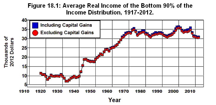
Where Did All The Money Go?
Chapter 19: Beyond the Current Crisis
George H. Blackford © 5/15/2013
Globalization, combined with technological improvements in transportation and communication over the past thirty years have led to incredible growth in productivity and output throughout the world. Unfortunately, this growth is derived from the same failed nineteenth century ideological paradigm of free-market capitalism that led to the deregulation of our financial system.
As we have seen, this paradigm is terribly flawed in its failure to understand the necessity to regulate financial markets or to understand the dependence of mass-production technologies on the existence of domestic mass markets. It is also terribly flawed in its failure to understand the necessity to regulate pollution and to preserve our natural resources.
Externalities in Free Markets
This nineteenth-century paradigm assumes that the quantities of goods and services produced are determined in markets through the interactions of buyers and sellers in such a way as to minimize the costs of producing while at the same time maximizing the benefits to society as a whole. The academic discipline of economics has provided a logically consistent and mathematically elegant model of market behavior that describes how this ideal system of human interaction is supposed to work as well as the prerequisites for the existence for such a system to actually work.
Unfortunately, the assumptions on which the logical consistency of this model depends—the most important being that no economic actor has the power to directly influence a market price, all market participants have perfect information as to the determination of all market prices, that there are no external costs or benefits associated with the production or consumption of any good, and that people behave rationally—are impossible to achieve in the real world.[19.1] The particular shortcoming of this model I wish to discuss here is the problem of externalities.
At the core of the economic theory that explains how the benefits to society as a whole are maximized in a market economy is the requirement that market prices reflect the costs to society as a whole that result from producing goods and services and that market prices also reflect the benefits to society as a whole that result from consuming the goods and services that are produced. This theory breaks down whenever there are costs or benefits that are external to the process of production or the act of consumption and, as a result, are not reflected in the market price. (Musgrave) To see how this breakdown occurs, consider the problem of disposing of the toxic waste generated in the process of producing chemicals.
A chemical company can minimize the cost it must pay—its private costs—to dispose of its toxic waste and, thereby, maximize its profits, by simply dumping its waste into the nearest stream or ditch. The polluted streams and aquifers that result threaten our supplies of potable water and cost society dearly. When a chemical company is able to externalize the costs of disposing of its toxic waste in this way, the private costs of producing chemicals are substantially less than they would be if the company had to pay these costs, and the true costs to society as a whole of the chemicals produced are not reflected in their prices. This leads to an over production of chemicals in the sense that if chemical companies had to pay the true costs of producing chemicals, which would include the cost of safely disposing of their toxic waste, the price they would be willing to sell chemicals for would be higher, less would be purchased, and less would be produced. (Smith Kuttner Musgrave)
What’s more, if chemical companies are not prevented by law from dumping their toxic waste, they will have no choice but to dump it because those companies that try to be socially responsible and dispose of their toxic waste safely will have higher costs than those that do not try to be socially responsible. As a result, socially responsible companies will be driven out of business by socially irresponsible companies as irresponsible companies drive market prices below the costs that must be paid by companies that try to dispose of their toxic waste responsibly.
In other words, chemical companies must be forced by the government to be socially responsible or they will be forced by the market to be socially irresponsible. That’s how markets work, and the only alternative to government intervention in the face of these kinds of external costs is to allow the external costs to destroy the environment on which the human race depends for its very existence.
This problem is, of course, not limited to the chemical industry. The cheapest way to produce electricity is by burning high sulfur coal and spewing the effluent into the atmosphere. The acid rain and concomitant deforestation of the planet that result are costs to society as a whole that are not reflected in the market price and are not borne by the producers or consumers of electricity in the absence of government regulation.
The cheapest way to run a nuclear power plant is to scrimp on safety, a practice which places enormous geographical regions at risk of utter devastation, the costs of which are not reflected in the market price of nuclear generated electricity and are not borne by the producers or consumers of nuclear generated electricity in the absence of government regulation.
The cheapest way to control pests in agricultural is through the use of long lasting, carcinogenic chemicals such as DDT which have devastating, long lasting consequences for human health and the environment, the costs of which are not reflected in the market price and are not born by the producers and consumers of agricultural products in the absence of government regulation.
The cheapest way to make paint or gasoline is by adding lead to the mix which spreads this toxic element throughout the environment, the costs of which are not reflected in the market price and are not born by the producers and consumers of paint or gasoline in the absence of government regulation.
The list of dangers to the environment from unregulated markets when there are external costs goes on and on, and the dangers are not confined to external costs of production. There can be external costs of consumption as well. The most obvious threat to the environment today is the buildup of greenhouse gases in the atmosphere that is leading to global warming. One of the largest sources of greenhouse gases is the carbon dioxide produced by burning gasoline in the internal combustion engines that power our automobiles. The threat to the planet is imminent, and there is no way markets can deal with this threat because it arises from the external costs of consuming gasoline, costs that are not reflected in the price of gasoline.
Since the price of gasoline does not come anywhere near reflecting the costs to the world community from driving our cars, consumers of gasoline do not have to pay these costs. Consumers of gasoline gain all of the benefits of cheap transportation while they destroy the ecological balance of the carbon cycle, and there is no market mechanism that can keep this from happening in the absence of government intervention. In fact, in the absence of government intervention, it is inevitable that the market must destroy the carbon cycle balance because it will always be cheaper and more convenient for most people to drive cars than to utilize more fuel efficient forms of transportation so long as those who drive cars have to pay only the private costs of producing gasoline and do not have to pay the social costs of consuming gasoline.
There exists no mechanism within a market system of economic organization to control the external costs of production and consumption in the absence of government intervention, and it is inevitable that a system of free markets that allows each individual and firm to force the rest of the world to pay these costs will eventually destroy itself if the government does not step in to keep this from happening.
Free Markets and Natural Resources
Not only does the nineteenth century ideological paradigm of unregulated free markets ignore the serious environmental problems that result from external costs, this paradigm also ignores the voracious appetites with which free markets devour natural resources. This aspect of free-market capitalism, along with the problem of pollution, was of little consequence in the nineteenth century when the world’s population was but a fraction of what it is today, when only a small fraction of world’s economy was industrialized, and when the vast majority of the world’s population lived a communal existence based on self sustaining, renewable technologies. The fact that a relatively small industrialized sector of the world community consumed natural resources at an accelerated rate and polluted the environment out of proportion to its size was of little consequence in such a world. This is not the case today.
Figure 19.1 plots the United Nations estimates of the world’s population from 1000AD through 2150. It should be clear from this plot that today’s world is dramatically different from what it was in the nineteenth century. The world’s population increased by 68% in the 100 years from 1800 to 1900 as it went from 980 million to 1.65 billion. In the next 50 years it increased by another 53% to 2.5 billion. It then increased dramatically as it went from 2.5 billion in 1950 to 6.06 billion by 2000, a 142% increase in just 50 years. Barring a worldwide economic catastrophe, the world’s population is expected to increase by another 50% in the next 40 years as it approaches 9 billion people by 2050. (UN Sachs)
Source: United Nations, The World at Six Billion.
Not only has the world’s population grown at an astounding rate over the past fifty years, the world’s output of goods and services has grown at an even more astounding rate, especially in recent years. As the world’s population increased by 11% from 1980 through 2010, its output of goods and services increased by almost 50%. At the same time the proportion of the world’s output produced by the advanced countries fell from 80% in 1980 to 67% in 2010. (UN)
This 16% drop in the contribution of the advanced countries to the total output of the world’s economy as total output increased by 50% is both gratifying and alarming. Gratifying because it means a larger portion of the world’s output is being produced by the less developed countries of the world with all of the potential that holds for the improvement in economic well being for the impoverished in those countries. At the same time it is alarming because that increase in output is based on a flawed economic paradigm that is unsustainable.
The tremendous increase in economic productivity and output that has made the remarkable increase in the world’s population possible over the past three-hundred years have come from technological advances that have allowed us to harness the energy stored in but three natural resources, namely, coal, oil, and natural gas. In the eighteenth and nineteenth centuries we mastered the technology of coal, and in the twentieth century we mastered the technology of oil and natural gas. Today’s economic system depends crucially on these three natural resources, especially oil, all of which are nonrenewable and all of which pose a serious threat to the environment.
As was noted above, this was of little consequence in the nineteenth century when the world’s population was relatively small and a relatively small sector was industrialized, but in the twenty first century with the world’s population approaching nine billion people and the entire world striving toward industrialization, the nonrenewable nature of our resources and the inevitable consequences of accelerating pollution cannot be ignored. The economic output of the world would have to increase by a factor of 3.5 over the next forty years to bring the rest of the world’s population up to the standard of living enjoyed by the advanced countries today even if there were no increase in the world’s population or in the standard of living in the advanced countries. The increase would have to be by a factor of 4.6 if the world’s population were to rise to the expected nine billion, and even more if the standard of living in the advance countries were to increase as well.[19.2] The math is irrefutable, and there is no way unregulated free markets are going to defeat this math.
With the incredible advances in transportation that have evolved over the past sixty years, combined with the unimaginable network of instant worldwide communication that came into being during the last twenty, the drive for industrialization in today’s world cannot be stopped. The concomitant effects on the environment and the limitations placed on development by the finite nature of our natural resources—specifically, oil but potable water as well—must be acknowledged and dealt with if widespread famine and starvation are to be avoided in the future. (Sachs)
Conclusion
In dealing with the problems of pollution and dwindling natural resources, free-market ideologues are in a state of denial. When it comes to global warming they argue 1) there is no such thing as global warming, 2) even though there is global warming it’s not our fault, and 3) if the government will just get out of the way free markets will solve the problem. (PRC) In dealing with the problem of preserving our natural resources they insist that the actions of free individuals in unregulated free markets that are free of government intervention will solve these problems without our having to worry about them.
It is worth keeping in mind, however, that these are the same people who deregulated our financial system, facilitated the concentration of monopoly power into the hands of larger and larger, too-big-to-fail institutions, guided our trade policies into continuing trade deficits and the outsourcing of our manufacturing sector, failed to enforce laws against fraud and unfair labor practices, and imposed a tax structure on the populace that is incapable of maintaining the public infrastructure and social capital from which those at the top of the income distribution have benefited so greatly—the same people whose policies undermined our mass markets and drove the world’s financial system to the brink of destruction. And these same free-market ideologues are now blaming “entitlement programs” for the economic catastrophe their policies have created as they block the tax increases needed to deal with the resulting deficit/debt problem and insist on cutting Social Security, Medicare, and other social-insurance programs in order to balance the federal budget.
Given this record, it is difficult to understand why anyone would take these people seriously, but, unfortunately, much of the electorate does take them seriously, as does the leadership of both the Republican and Democratic parties.
Over the past thirty years free-market ideologues have been able to block virtually every attempt to deal with the problems posed by rapidly rising external costs brought about by rapidly increasing population and economic growth in a world economy fueled by nonrenewable natural resources. Their influence in the United States has led to Carter’s energy program being dismantled in the 1980s, CAFÉ standards that barely changed after 1984 until gasoline prices peaked in the mid 2000s, funding for the cleanup of superfund toxic waste sites being allowed to expire in 1995, the United States walking away from the Kyoto Protocol on global warming in 2001, and water pollution restrictions being reduced in 2003. (Hartmann NHTSA GAO Time CSM)
Their continued success in this regard does not bode well for the future. Aside from the problem of global warming, the transportation and agricultural systems we have developed as a result of modern technology depend crucially on oil. These systems have led to incredible increase in productivity over the past fifty years, but in the face of increasing world population and economic growth this technology is unsustainable.
As world oil reserves dwindle and the demand for oil increases, the price of oil must increase, and, in turn, the productivity of our transportation and agricultural systems must decline. Until we are able to find a renewable source of energy to replace oil, prospects for the future are dim. In the meantime, it is going to become more and more difficult to feed the world’s population, and a rise in conflict, political instability, and turmoil throughout the world is inevitable. (EB)
If we value the kind of world we leave to our children and grandchildren we cannot sit back and hope for the best as unregulated markets squander our natural resources and pollute our planet. The problems posed by population growth, the drive to industrialize, and the finite nature of our natural resources cannot be solved by markets alone. They can only be solved through the international cooperation of governments. (Sachs)
Endnote
[19.1] It is, perhaps, worth noting that this fact is well known and well understood within the discipline of economics and is accepted by virtually all who know anything at all about the discipline or about the world in which we actually live. It’s not open to debate except, of course, among those who are either completely out of touch with reality or who make their living by denying this fact.
[19.2] These estimates are derived from the following table taken from the International Monetary Fund, World Economic Outlook Database:
Country Group Name
Subject Descriptor
Units
Scale
2010
Adv. economies
GDP(PPP)
Cur.Int.dollar
Billions
38,693.78
Adv. economies
GDP(PPP)/capita
Cur.Int.dollar
Units
38,024.65
Adv. economies
Population
Billions
1.01
Emrg. & dev. economies
GDP(PPP)
Cur.Int.dollar
Billions
34,505.83
Emrg. & dev. economies
GDP(PPP)/capita
Cur.Int.dollar
Units
5,953.64
Emrg. & dev. economies
Population
Billions
5.80
where population is estimated by dividing GDP(PPP) by GDP(PPP)/capita.
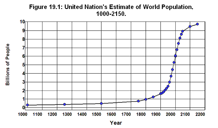
Where Did All The Money Go?
Acknowledgements / Autobiographical Information
I was born on August 28, 1942 in Flint, Michigan. The earliest childhood memory I can date was August 14, 1945. I was standing with my mother in front of our house on Edmond St. and asked her why all the cars were blowing their horns. She look down at me and said "Because the War is over." My next earliest memory was November 30 of that year when my father came home from the Army. All of my family in my parents' generation served in that war—my father and uncles in the military, my mother and aunts in the in the factories. The experiences of my parents' generation during the war, and during the depression that preceded the war, have had a profound effect on my view of the world throughout my life.
I have been married twice, and raised six children—five daughters and one son—the oldest of which is 52 and the youngest 27. I have eight grandchildren and five truly amazing great grandchildren. No one really expects to have great grandchildren until it happens!
I am what I would call a state-school economist. I graduated from the University of Michigan-Flint in 1966 and received a Masters Degree in economics from the University of Michigan-Ann Arbor in 1967. I taught economics for a year at Ferris State College in Michigan as an instructor. I then entered the Ph.D. Program in economics at the State University of New York at Buffalo where I taught economics in the night school for three years. In 1972 I moved to Potsdam, NY and taught at the Potsdam state college for a year then returned to Buffalo in 1973 and taught at the Buffalo state college until 1979. I received a Ph.D. in economics from the State University of New York at Buffalo in 1974. My dissertation was in monetary and macro economic theory.
In 1979 I moved back to Flint to chair the Department of Economics at the University of Michigan-Flint and taught there until 1987. I also taught a year at GMI Engineering & Management Institute, now known as Kettering University. I then put together a statistical package, left academia and began selling my statistical package to colleges and universities and to publishers as a supplement to statistics textbooks. Other than my statistical package and its manuals, my publication record is sparse—one article in the Eastern Economic Journal, a note in the Journal of Political Economy, and a number of papers on monetary and macroeconomic theory in various papers and proceedings.
I spent the twenty years leading up to the crisis in 2008 reading mostly mathematics and statistics books and paid very little attention to the real world other than to watch the news. The financial crisis took me entirely by surprise. I knew there was a problem in the housing market and that economic nonsense had been at the center of the political debate in our country for over thirty years, but I assumed, naively it turned out, that cooler heads would prevail, and sound economic policies would always be enforced. I had no idea the extent to which ideological beliefs had taken over the discipline of economics since I left academia or that our financial institutions would be allowed to overextend themselves to such an extent they could bring down the economy of the entire world.
After the crash in 2008 I decided to set aside other pursuits and try to find out what had been going on in the world of economics since I left academia. I read virtually everything I could get my hands on relating to the financial crises in an attempt to understand how we got to where we are today. The result is the collection of papers in Where Did All the Money Go? and those posted on my www.rwEconomics.com website.
It will be apparent in some of the essays that my academic interests go beyond economics to history, political science, psychology, and philosophy. I attribute these interests to a two year, twenty credit hour Western Civilization program offered at Alma College, which I attended as a freshman and sophomore, and to a number of very talented and highly dedicated teachers I had the privilege of being influenced by in my tender years. Alma’s Western Civilization program was team taught and most of the faculty participated in the program. It provided an integrated, interdisciplinary and comprehensive view of the cultural, political, and economic evolution of our 10,000 years of history that was truly remarkable. Sadly, this program is no longer offered today.
As for the very talented and highly dedicated teachers I had the privilege of being influenced by, I would like to take the opportunity to acknowledge them here: In grade school: Mrs. Shegus, Mrs. Lockner, and Miss Fortiner. In junior high: Neil Cason. In high school: Charles Shinn, Joseph T. Davis, William H. Whitemore, and Barbara and Robert Anderlik. In college: Frank Jackson, William M. Armstrong, Florence A. Kirk, Louis R. Miner, Louis Toller, Alfred C. Raphelson, Elston W. Van Steenburgh, Paul G. Bradley, and Virgil M. Bett. In graduate school: W. H. Locke Anderson, Daniel B. Suits, Kenneth E. Boulding, Saul H. Hymans, Mitchell Harwitz, Cliff L. Lloyd, Ray Boddy, James Crotty, Winston Chang, and Nagesh S. Revankar. Each of these individuals had a profoundly positive influence on my life, and I will be indebted to each forever.
My indebtedness goes beyond academia, of course, and especially to my family. My wife, Dolores M. Coulter, has been a pillar of strength in our relationship for over thirty years. I would be lost without her. I am also indebted to my two sisters, Kathy J. Ross and Gay S. Towfiq, and to my brothers and sisters in-law, James Ross, Basim Towfiq, Melissa and Mark Scharrer, Mary Cerreto and David Coulter, Theresa Coulter, Malcolm Coulter, and Gordon C. FitzGerald as well as my former wife, Karen F. Blackford. All are more than family, but friends that have always been there to do what they could when the need arose. Then there are the cousins, spread throughout the country and too numerous to mention or even keep track of, all of whom provide a sense of belonging and connectedness in this isolated world.
I am particularly indebted to the generations that came before, especially to my grandparents, Mary and Henry White and Juanita and George Blackford, as well as grandpa Hendrick L. Adams and grandma Delia Coulter, and to my great aunts and uncles, Grace Cuvrell, Louise and Enoch Anderson, Minnie and Joe Baumgartner, Cecil and Will Baumgartner, Louie Baumgartner, and Lizzie and Rudolph Baumgartner. They led remarkable, hardworking, and honorable lives and set sterling examples for me to live up to, as did my parents, Marion R. and George P. Blackford, and my fathers and mothers in-law, Eunice and Cecil W. FitzGerald and Helen and Malcolm Coulter.
The same is true of my aunts and uncles: Oliver White, Cecil and Frank Pugh, Lois and Thomas Shinas, Carol and Charles Cardwell, Donna and David Cuvrell, Marsha and Louis Irwin, Marjorie and Dick Blackford, Yvonne and William Finley, and Marilyn and Gene Glanton. I have not always been able to live up to the examples they set, but I will be forever grateful their examples were there for me to look up to, to admire, and to strive for.
Then there are the kids: Heidi, Steve, Robin, Theresa, Cherilyn, Brad, Terri, Mark, Leigh, Bobby, Sandy, Chelsea, Jeremy, Cynthia, Jason, Stephanie, Shannon, Joe, Stevie, Elizabeth, Ed, Jessica, David, Ryan, Andrea, Ashley, Tauri, Shawna, Maria, Anna, Caley, Sam, Emma, Alex, Aidan, Lucas, Joey, Sophia, Maxwell, Lily, and Brily. What does it all mean without them? It is for them that I posted my website in the hope it will contribute toward a better understanding of the world in which we live and toward a better future for all our children.
I wish to thank those who have directly and indirectly contributed to this website: Harry Frank, Gillian Garcia, Rajindar Koshal, G. William Domhoff, Douglas J. Amy, James DiGiacinto, Nick Seraphinoff, Paul O’Brien, my wife Dolores, sister Kathy, brother-in-law Jim, sister-in-law Mary, niece Cherilyn, daughter Elizabeth, granddaughter Shannon, grandsons Jason, Ryan, and Stevie, brother-in-law Malcolm, and my uncle Gene for their constructive criticisms of the ideas contained in earlier drafts of various papers. This is especially so for my uncle Gene who was particularly conscientious in responding to my pleas for help before he passed away in October of 2009. His friend, Robert Maximoff, described my uncle best with the quote from Shakespeare: "His life was gentle, and the elements so mixed in him that Nature might stand up and say to all the world, 'This was a man.'" He was a very good man and is deeply missed by all who knew him.
I also wish to thank Gloria McIntyre Zucker, Gail Rodd, Doris Suciu, Jim Hoffmeister, Robert Maximoff, my Aunt Marjorie and Uncle Dick, and my nephews Bobby and Brad for the encouragement they have given me.
Finally, I wish to thank Karl Agcaoili, Hugh Connelly, Tobias Adrian, Patrick Locke, Adrienne Pilot, Bob Rand, and Benjamin Mandel for the assistance they have given me in sorting through government data sources.


![]()
Where Did All The Money Go?
Selective Bibliography
![]()
Amazon.com publishes reviews by readers that give you some idea what others think of each book. The links to books below take you to these reviews, whenever they are available. The author's name is generally linked to an online biography.
Acharya, Viral and Matthew Richardson (Editors), Restoring Financial Stability: How to Repair a Failed System (2009) is a collection of papers written by the faculty of the New York University Stern School of Business that explain the fundamental causes of the current financial crisis and offers proposals as to how to prevent such crises in the future.
Akerlof, George and Robert J. Shiller (2009) Animal Spirits: How Human Psychology Drives the Economy, and Why It Matters for Global Capitalism examines the role of confidence in causing depressions.
Alperovitz, Gar and Lew Daly, Unjust Deserts: How the Rich Are Taking Our Common Inheritance (2008) examines the contribution of what we have inherited from the past to our ability as individuals to produce wealth in the present.
Altemeyer, Bob, The Authoritarians (2006) examines the scientific research pertaining to the personal beliefs actions of those people who are particularly susceptible to rightwing propaganda as well as those of the leaders of right-wing movements. He relates this research to the history of rightwing movements the 1930s as well as to the rightwing movements today. Most important, he explains why these movements pose a threat to our freedom and to the very existence of our democratic society.
Amy, Douglas J., Government is Good: An Unapologetic Defense of a Vital Institution (2010) provides a comprehensive discussion of the role of government in providing for the common good in society that explains why strong government is essential to our economic wellbeing and individual freedom and liberty. Amy's work provides a lesson in civics that the American electorate desperately needs.
Bair, Sheila A., Bull by the Horns: Fighting to Save Main Street from Wall Street and Wall Street from Itself (2012) not only examines the interactions between the regulatory agencies during the financial crisis, but provides an exceedingly good explanation of the problems that led to the crisis, and the kinds of regulatory changes needed to avoid this kind of crisis in the future.
Baker, Dean, Taking Economics Seriously (2010) examines how economic are being misused and how they should be used to deal with economic problems .
———, Plunder and Blunder: The Rise and Fall of the Bubble Economy (2009) explains the nature of speculative bubbles, why speculative bubbles have become such an endemic part of our economic system over the past thirty years, and how the housing bubble led to the crisis of 2008.
———, and Mark Weisbrot, Social Security: The Phony Crisis (1999) explains why there is no economic or demographic crisis that requires the dismantling of the Social Security System.
Bernanke, Ben S., Essays on the Great Depression (2000) provides a collection of essays on the causes and nature of the Great Depression from a Neoclassical perspective. It also examines the role of the Gold Standard in the international transmission of the economic collapse among countries.
Black, William K., The Best Way to Rob a Bank Is to Own One: How Corporate Executives and Politicians Looted the S&L Industry (2005) provides an in depth look at the savings and loan crisis of the 1980s.
Bogle, John C., Enough: True Measures of Money, Business, and Life (2009) examines the breakdown in business ethics that has accompanied the government deregulation of the economic system over the past thirty years.
———, The Battle for the Soul of Capitalism by (2005) examines the transformation of the American capitalist system from owner's capitalism where stock owners control corporations to manager's capitalism where managers control corporations. This book makes an extremely important contribution to the understanding of how today's economic system works.
Bookstaber, Richard, A Demon of Our Own Design: Markets, Hedge Funds, and the Perils of Financial Innovation (2007) examines the role of market complexity in risk management and economic instability.
Boyer, Richard O. and Herbert M. Morais, Labor's Untold Story (1979) tells the story of the labor movement from the prospective of the union organizers.
Bruner, Robert F., The Panic of 1907: Lessons Learned from the Market's Perfect Storm (2007) provides a comprehensive examination of the financial crisis of 1907 that led to the founding of the Federal Reserve System in 1913.
Buchanan, James M., and Richard A. Musgrave Public Finance and Public Choice: Two Contrasting Visions of the State (2004) provides a valuable insight into the way in which the fundamental issues surrounding the free market ideology have been debated within the discipline of economics.
Carson, Rachel, Silent Spring (1962) examined the effects of pollution on the environment in the United States.
Carville, James and Paul Begala Take It Back: Our Party, Our Country, Our Future (2008) discusses some of the consequences of the rise of Free Market Movement in the United States over the past forty years and the failure of the Democratic Party to confront these consequences.
Cassidy, John, How Markets Fail: The Logic of Economic Calamities (2009) is the most uneven book I have ever read. Part I provides an excellent discussion of the failings of Utopian Economics, Part II provide an adequate discussion of Reality-Based Economics, and Part III contains so many misstatements, misunderstandings, and outright falsehoods that it appears to have been written by someone other than the person who wrote Part I. I do not recommend reading this book beyond Chapter 16.
Chandrasekaran, Rajiv, Imperial Life in the Emerald City: Inside Iraq's Green Zone (2006) documents the role that ideological bias played in the ineptitude, incompetence, and corruption played in our attempts at nation building in Iraq. When read in conjunction with Naomi Klein’s book, The Shock Doctrine, it would appear that this ineptitude and incompetence may have been intentional.
Chriss, Neil A., Black-Scholes and Beyond: Option Pricing Models (1997) explains the Black-Scholes model of option pricing and the way this model has been extended to handle the pricing of other derivatives.
Cohan, William D., House of Cards: A Tale of Hubris and Wretched Excess on Wall Street (2009) tells the story of the fall of Bear Stearns.
Cooper, George, The Origin of Financial Crises (2008) examines the role of the rational/efficient market fallacy of the Chicago School in deregulating the financial markets and generating the housing crises.
Derman, Emanuel, My Life as a Quant: Reflections of Physics and Finance (2005) examines the role played by mathematicians, physicists, and other quantitative types on Wall Street from1985 through 2005.
Domhoff, G. William, Who Rules America? (1967) is the first in a series of books by Domhoff that examine the power structure in America and explains how that power structure maintains control within our society. Much of Domhoff's analysis is explained on his website, http://sociology.ucsc.edu/whorulesamerica/
———, Who Rules America Now? A View From the 80s (1986) is an update of Domhoff's 1967 book that examines the changes in the power structure that took place in the 1970s and early 1980s.
———, The Myth of Liberal Ascendancy: Corporate Dominance from the Great Depression to the Great Recession (2014) is a truly remarkable book in which Domhoff examines in great detail the way in which the conservative political collation in the United States has dominated American economic policy since 1939.
Dowd, Kevin and Martin Hutchinson, Alchemists of Loss: How Modern Finance and Government Intervention Crashed the Financial System (2010) provides an account of how institutional changes led to perverse incentives and short-rum, optimizing behavior that, when combined with naive risk models and a misguided belief in the efficiency of markets ultimately led to excess risk taking and inevitably to a collapse of the system. The authors attempt to explain all of this in terms of government meddling with the economy in spite of the fact that the prelude to this crisis was twenty odd years of deregulation in which the government refused to meddle in the markets.
Durbin, Michael, All About Derivatives (2006) provides a basic introduction to derivatives, what they are, how they are priced, and how they are used.
Eichengreen, Barry, Exorbitant Privilege: The Rise and Fall of the Dollar and the Future of the International Monetary System (2011) examines the role of the dollar in international finance and trade and explains why the US financial crisis has not yet led to an international exchange collapse and what could cause this situation to change.
———, Golden Fetters: The Gold Standard and the Great Depression, 1919-1939 (1995) examines how the functioning of the post World War I gold standard contributed to the Great Depression of the 1930s.
Ferrara, Peter J., Social Security: The Inherent Contradiction (1980) is an example of the schizophrenic nature of ideological logic. In the course of trying to prove the inherent contradiction of attempting to serve a welfare function within the context of an insurance program, Ferrara unwittingly provides a compelling argument for eliminating the income cap on payroll taxes and extending Social Security taxes to unearned income. His argument that the pay-as-you-go nature of Social Security reduces economic growth depends crucially on the dubious (I would say absurd) assumption that an increase in saving forces investors to invest. At the same time, his seemingly irrefutable math/logic that Social Security beneficiaries would be better off if they were to put their payroll tax money in private investment accounts is oblivious to the risks involved in this scheme and the dismal history of private retirement accounts and pension funds going broke.
Farmer, Roger E. A., Expectations, Employment, and Prices (2010) an original work that attempts to integrate modern macroeconomic theory with Keynes's theory of expectations.
FCIC, The Financial Crisis Inquiry Report, Authorized Edition: Final Report of the National Commission on the Causes of the Financial and Economic Crisis in the United States (2011) provides an in depth examination of the 2008 financial crisis.
FDIC, History of the 80s, (1997) provides an insightful analysis of the regulatory failures that led to the financial crisis of 1988. Again, it is astounding how the Bush Administration either ignored or was completely oblivious to principles explained in this book. This book can be read on line by clicking on one of the above links.
Fisher, Irving, Booms and Depressions (1932) provides the first explanation as to how excess leverage inspired during an economic boom leads to financial crises and economic collapse in a capitalistic system.
Fox, Justin, The Myth of the Rational Market: A History of Risk, Reward, and Delusion on Wall Street (2009) examines the history of the rational/efficient market hypothesis as it was created by the free market ideologues in the utopian world of the Chicago School of Economics.
Frank, Thomas, The Wrecking Crew: How Conservatives Rule (2008) explains the role of the Free Market Movement in the rise of the Republican Party from the Goldwater defeat in 1964 through the present and explains the role of each of the participants and factions in this rise, including the role played by Jack Abramoff from the 1970s onward.
———, What’s the Matter With Kansas: How Conservatives Won the Heart of America (2004) explains how the Rightwing Propaganda Machine was able to shift the body politic to the right in Kansas.
Freeman, Joshua B., Working-Class New York: Life and Labor Since World War II (2000) presents a history of New York City since World War II in which he examines the effects of the policies discussed by Tabb through to 2000.
Friedman, Milton and Rose Friedman, Free to Choose: A Personal Statement (1980) is a well written explanation of Friedman’s view of the benefits of free market capitalism. It combines an insightful analysis of the inefficiencies of government interference with markets with an appalling lack of insight as to the harm caused by market failures in the lives of ordinary people.
——— and Anna Jacobson Schwartz, A Monetary History of the United States, 1867-1960 (1971) is a well written tome that provides a comprehensive history of the financial system in the United States.
——— and Anna Jacobson Schwartz, The Great Contraction, 1929-1933 (1963) is also a rather short, very well written history of the stock market crash of 1929 and its aftermath.
———, Capitalism and Freedom (1962) provides an explanation of Friedman’s view of the relationship between free market capitalism and his concept of freedom.
Galbraith, James K., Inequality and Instability: A Study of the World Economy Just Before the Great Crisis (2012) examines the role of inequality in increasing unemployment and economic instability.
———, The Predator State: How Conservatives Abandoned the Free Market and Why Liberals Should Too (2008) examines the institutional changes in the world economy that have taken place over the past sixty years and suggests a plan to deal with the disastrous consequences that have resulted from the free market economic policies of the past thirty years.
Galbraith, John Kenneth, The New Industrial State (1966) examines the role of technology, technocrats, and government within the modern economic system.
———, The Affluent Society,(1958) examines the way in which the power structures within the economic system develop and counterbalance each other.
———, The Great Crash of 1929 (1955) is a rather short, very well written history of the stock market crash of 1929 and its aftermath.
Garcia, Gillian, Carl-Johan Lindgren, and Matthew I. Saal, Bank Soundness and Macroeconomic Policy (1996) provides a comprehensive analysis of the kinds of problems faced by financial regulators throughout the world and the kinds of regulatory policies that are essential for effective regulation of the financial system. It is astounding how the Bush Administration either ignored or was completely oblivious to the principles explained in this book.
Gasparino, Charles, The Sellout: How Three Decades of Wall Street Greed and Government Mismanagement Destroyed the Global Financial System (2009) is a somewhat uneven account of the of the history of the financial system over the past thirty years in the sense that his grasp of basic economics in some areas is lacking (he sees the FDIC as bailing out banks and the GSEs as guaranteeing mortgages, which indicates a fundamental misunderstanding of these institutions). Other than that Gasparino's history of this period is quite good. It is fairly comprehensive, objective, and surprisingly, for the most part, non-ideological.
Gelinas, Nicole, After the Fall: Saving Capitalism from Wall Street and Washington (2009) provides a concise statement of the kinds of regulations that are necessary to avoid future financial crises. Specifically, she argues that the principles of regulation needed today are the same as those put in place in the 1930s which allowed us to avoid financial crises for fifty odd years until they were dismantled beginning in the 1970s. These principles include limiting speculative bowering by imposing margin/capital requirements, requiring full exposure on the part of financial intuitions, and circumscribing reckless exposure to risk on the part of these institutions.
Graeber, David, Debt: The First 5,000 Years (2010) is a fascinating history of debt, its relationship to money, and the role it has played throughout history. This is a very important book.
Harrington, Michael, The Other America: Poverty in the United States (1962) examined poverty in the United States.
Hartmann, Thom, Cracking the Code: How to Win Hearts, Change Minds, and Restore America's Original Vision (2008) provides a very well written nonacademic explanation of the framing mechanism.
———, Screwed: The Undeclared War Against the Middle Class - And What We Can Do about It (2007) discusses some of the consequences of the rise of free market capitalism in the United States over the past forty years.
Harvey, David, A Brief History of Neoliberalism (2005) discusses the hypocrisy endemic in the Free Market Movement in terms of what is called Neo-Conservatism in the United States and Neoliberalism in the rest of the world. This book documents the way in which the policies of free market ideologues when implemented in the name of freedom and economic prosperity for all have lead to freedom and economic prosperity for the few and desperation for most everyone else.
Hayek, Friedrich von, The Road to Serfdom (1944) has proved to be one of the seminal documents of the Free Market Movement. It provides the basis for the argument that government intervention in markets leads to totalitarian socialism. A Reader’s Digest condensed version of this book is available on line.
Haywood, William, Autobiography of "Big Bill," Haywood (1966) tells the life story of Big Bill Haywood and his involvement in the labor movement in founding the Western Federation of Miners and the International Workers of the World during the latter half of the nineteenth century.
Heilbroner, Robert, The Worldly Philosophers: The Lives, Times And Ideas Of The Great Economic Thinkers (1955-1999) is the place to start. This book provides a history of economic thought throughout the nineteenth and twentieth centuries, and has gone through seven additions.
Henriques, Diana B., The White Sharks of Wall Street: Thomas Mellon Evans and the Original Corporate Raiders (2000) examines the beginnings of the hostile takeover and leverage buyout craze leading up to the 1980s.
Huntington, James B., Work's New Age: The End of Full Employment and What It Means to You (2011) examines the problems automation creates in maintaining full employment in today's world.
Isikoff, Michael and David Corn, Hubris: The Inside Story of Spin, Scandal, and the Selling of the Iraq War (2006) documents the way in which the Bush Administration distorted available intelligence in order to justify their invasion of Iraq.
Johnson, Haynes, The Age of Anxiety: McCarthyism to Terrorism (2006) shows the similarities between the tactics used in the McCarthy Era and those used by the Rightwing Propaganda Machine today.
Johnson, Simon and James Kwak, White House Burning: The Founding Fathers, Our National Debt, and Why it Matters to You (2012) examines the his history of the federal debt and explains the fundamental choices we are faced with today in dealing with our federal deficit/debt problem.
———, 13 Bankers: The Wall Street Takeover and the Next Financial Meltdown (2010) compares the way financial crises are dealt with in third world countries and how we dealt with the crisis of 2008.
Jones, Mary Harris and Mary Field (editor) , The Autobiography of Mother Jones (1996) tells the life story of Mother Jones and her involvement in the labor movement during the latter half of the nineteenth century.
Josephson, Matthew, The Robber Barons (1934) is, of course, the classic work describing the excesses of free market capitalism in the latter half of the nineteenth century.
Kennedy, David M., Freedom from Fear: The American People in Depression and War, 1929-1945 (1999) provides an in depth account of the ways in which the Great Depression and World War II changed the American society from 1929 through 1945.
Keynes, John M., The General Theory of Money, Interest, and Prices (1936) (Electronic Edition) is the classic work on the economics of depressions.
Kindleberger, Charles P. The World in Depression, 1929-1939: Revised and Enlarged Edition (History of the World Economy in the Twentieth Century) (1986) is a comprehensive examination of the Great Depression from the perspective of how it reverberated throughout the world.
———, and Robert Aliber, Manias, Panics, and Crashes: A History of Financial Crises (2005) provides an update to MacKay's tome and is much easier to read.
Kirk, Russell, The Conservative Mind: From Burke to Eliot (1953-1985) explains the conservative movement in the United States and England from the eighteenth century through the mid 1980s in terms of 1) an abiding faith in Natural Law as determined by a Devine Providence, 2) the superiority of intuition, predigests, and tradition over the scientific method in the search for meaning and truth, and 3) the belief that ideas are more important than facts in this regard. Unfortunately, Kirk fails to explain how a movement which he shows to have fought the spread of Free Market Capitalism and Democracy for over one hundred and fifty years has managed to become the unquestioning, fanatical champions of these two institutions in today's world.
Klein, Naomi, The Shock Doctrine: The Rise of Disaster Capitalism (2008) is probably the most shocking book I have ever read. It explains the role free market ideologues have played in international finance over the past forty years, and documents the disastrous consequences of their policies throughout Latin America, Eastern Europe, Indonesia, Iraq, and South Africa.
Krugman, Paul, The Great Unraveling: Losing Our Way in the New Century (2009) chronicles the economic misdeeds of the Bush Administration .
——— The Return of Depression Economics and the Crisis of 2008 (2009) examines the historical context in which the current financial crisis occurred and the underlying economics that brought this crisis about.
——— The Conscience of a Liberal (2007) discusses the way in which the Rightwing Propaganda machine is organized and the economic effects of this take over of the Republican Party on our society.
——— Peddling Prosperity: Economic Sense and Nonsense in an Age of Diminished Expectations (1995) explains the economic sense and nonsense generated by the Rightwing Propaganda Machine.
Kuhn, Thomas, The Structure of Scientific Revolutions (1962) presents, what was at the time Kuhn published this book, an iconoclastic explanation of the way in which scientific truth changes over time.
Kuo, David, Tempting Faith: An Inside Story of Political Seduction (2006) discusses the hypocrisy with which free market ideologues have used the Christian Right for their political and economic ends.
Kuttner, Robert, The Squandering of America: How the Failure of Our Politics Undermines Our Prosperity (2008) is a sequel to his Everything for Sale that examines the role the deregulation of economic behavior has played in undermining democratic institutions. He shows how giving lip service to the Utopian Capitalist's ideals has led to the squandering of America's economic resources and the concentration a larger and larger portion of our wealth and income in the hands of fewer and fewer people, and how this concentration of wealth and power has undermined the wellbeing of the vast majority of Americans.
———, Everything for Sale: The Virtues and Limits of Markets (1999) provides a devastating critique of the economic foundations of the free market ideology. It is one of the best, and most important books on the discipline of economics I have read. Anyone who considers herself an economist, or who has even a passing interest in the discipline of economics should read this book. Only the most ardent true believer in the free market ideology can fail to grasp its significance.
Lakoff, George, The Political Mind: Why You Can't Understand 21st-Century American Politics with an 18th-Century Brain (2008) explains the mechanism by which the Rightwing Propaganda Machine frames the political debate in our country to divert the debate from substantive issues to non-substantive issues within the context of the cognitive sciences.
———, Whose Freedom?: The Battle Over America's Most Important Idea (2006) explains the mechanism by which the Rightwing Propaganda Machine frames the fundamental concept of freedom to engender support for their agenda.
———, Don't Think of an Elephant: Know Your Values and Frame the Debate--The Essential Guide for Progressives (2004) provides a nonacademic explanation of the framing mechanism of the Cognitive sciences.
Lansley, Stewart, The Cost of Inequality: Why Economic Equality is Essential for Recovery (2012) examines the effects of inequality on the British economy with comparisons with the United States.
Levin, Carl and Tom Coburn, Wall Street and the Financial Crisis: Anatomy of a Financial Collapse (2011) provides both a comprehensive overview of the financial crisis and a detailed analysis of some of the major actors that helped to bring on this crisis.
Levitt, Arthur, Take on the Street: How to Fight for Your Financial Future (2002) examines the regulatory issues at the SEC during Levitt's tenure as Chairman of the SEC from 1993 through 2000.
Lewis, Michael, Liar's Poker: Rising Through the Wreckage on Wall Street (1989) examines the effects of deregulation during the 80s on the behavior of the financial sector as it led to the savings and loan crisis in the late 80s.
———, The Big Short: Inside the Doomsday Machine (2011) chronicles the events leading up to the Crash of 2008 through the eyes of a number of investors who saw it coming and shorted the market to make money off the crash.
Lindert, Peter H., Growing Public: Social Spending and Economic Growth Since the Eighteenth Century Volume 1 and Volume 2 (2005) provides a compelling history and analysis of the evolution of social welfare/transfer systems over the past three-hundred years. Volume 2 examines the statically analysis on which Lindert's conclusions are based.
Lowenstein, Roger, The End of Wall Street (2010) examines the housing bubble from its inception through the crash of 2008.
———, Origins of the Crash: The Great Bubble and Its Undoing (2004) examines the effects of deregulation on the dotcom and telecom bubbles during the 1990s and early 2000s.
———, When Genius Failed: The Rise and Fall of Long-Term Capital Management (2002) examines the effects of deregulation during the collapse of the Long-Term Capital Management hedge fund and the way in which it threatened to take down the entire financial system.
Lowndes, Joseph E., From the New Deal to the New Right: Race and the Southern Origins of Modern Conservatism (2009) examines the mechanisms by which southern conservatives took over the Republican party.
Lux, Michael , The Progressive Revolution: How the Best in America Came to Be (2009) examines the history of the Progressive movement in the United States.
Mayer, Jane, The Dark Side: The Inside Story of How The War on Terror Turned into a War on American Ideals (2008) documents the way in which the free market ideologues of the Bush Administration subverted the American government into adopting a policy of torturing people to serve their ends. It is very explicit in its discussion of the kinds of torture techniques used, the extent to which these techniques were used, and on whom these techniques were used. I do not recommend that everyone read this book. It is very upsetting.
MacKay, Charles, Extraordinary Popular Delusions and the Madness of Crowds (1841) is, of course, a classic tome on the subject of economic bubbles and other kinds of mass delusions. Unfortunately, it is rather dry reading and not nearly as fun as its title suggests.
Meltzer, Allan H., A History of the Federal Reserve, Volume 1: 1913-1951 (2003) examines the history of central banking and of the Federal Reserve through 1951.
Miller, T. Christian, Blood Money: Wasted Billions, Lost Lives, and Corporate Greed in Iraq (2006) documents the conflicts of interests and the huge fortunes that were made through political patronage in Iraq.
Minsky, Hyman P., Stabilizing an Unstable Economy (1986/2008) extends Keynes and Fisher's explanations of the Great Depression and explains how economic and psychological forces in the financial sector has a destabilizing effect on the economy in a capitalistic system. It is one of the most underrated books, until recently, in economics.
Mises, Ludwig von, Human Action: A Treatise on Economics (1949) is also a seminal document of the Free Market Movement. This tome provides the “praxeological” arguments for the notion that the underlying assumptions of the free market ideology are universal truths and explains why all that is good in the world comes from free markets and everything that is bad comes from interfering with free markets. This book is available on line.
Morris, Charles R., The Two Trillion Dollar Meltdown: Easy Money, High Rollers, and the Great Credit Crash (March 2008) explains the housing bubble and its bursting in 2007 and forecasted the crash of 2008 six months before it happened. Morris explained in detail why the coming crash was inevitable.
———, Money, Greed, and Risk: Why Financial Crises and Crashes Happen (1999) examines both the history and the economics of financial crises and evaluates the inadequacy and the importance of regulation in moderating these crises.
Musgrave, Richard, The Theory of Public Finance: A Study in Public Economy (1959) is a classic work on the functions of government in the economic system.
Nader, Ralph, Unsafe At Any Speed The Designed-in Dangers of the American Automobile (1965) chronologies the safety problems in the American automobile industry.
Orwell, George, 1984 Nineteen eighty four (1948) seems to provide both a warning and a guide to the free market movement: A warning as to the evils of totalitarian socialism, and a guide as to how to rule and control public opinion in a free market society.
Palley, Thomas I., The Economic Crisis: Notes From the Underground (2012) examines the causes of the economic crisis and the failure of the economics profession to foresee and explain it.
Patterson, Scott, The Quants: How a New Breed of Math Whizzes Conquered Wall Street and Nearly Destroyed It (2010) explores the role of hedge funds, quantitative models, and the belief in self-adjusting free markets in the meltdown of the economic system from 2007 through 2008. Provides some insight into the way electronic trading works in the global economy.
Perino, Michael, The Hellhound of Wall Street: How Ferdinand Pecora's Investigation of the Great Crash Forever Changed American Finance (2010) explains the importance of the Pecora Hearings in bringing about the financial regulation of the 1930s.
Phillips, Kevin P., Bad Money: Reckless Finance, Failed Politics, and the Global Crisis of American Capitalism (2008) provides a penetrating analysis of the way in which the rise of speculative finance combined with the geopolitics of oil and the failure of domestic politics in the United States to meet the challenge of state capitalism in the developing world led to the economic crisis with which we are faced.
———, Wealth and Democracy: A Political History of the American Rich (2002) provides an encyclopedic examination of the rise and fall of the Spanish, Dutch, and British empires and the striking similarities with the development of the United States' empire over the past 200 years.
———, The Emerging Republican Majority (1969) provides a comprehensive analysis of the changes in the voting trends through the 1968 election that eventually led to the Republican majority in the country.
Polanyi, Karl, The Great Transformation (1944) provides a critical view of the fundamental assumptions that underlie the Utopian Capitalist’s view of reality. The uniqueness of this book and its insight into the human condition makes it one of the most important, if not the single most important contribution to this debate. Unfortunately, it has received very little recognition within the discipline of economics.
Rajan, Raghuram G., Fault Lines: How Hidden Fractures Still Threaten the World Economy (2010) I a very disappointing book. While it contains some understanding of the current crisis, it contains innumerable ideological clichés and indicates a fundamental misunderstanding of the role government housing played in this crisis.
——— and Luigi Zingales, Saving Capitalism From the Capitalists: Unleashing the Power of Financial Markets to Create Wealth and Spread Opportunity (2003) argues for the need to regulate the financial markets.
Rand, Ayn, Atlas Shrugged (1959) concludes with the utopian dream of the Utopian Capitalists—a world without government where we all just get along.
Reich, Robert, Aftershock: The Next Economy and America's Future (2010) examines the consequences of the current crisis and argues that the long run effect of this crisis is going to be sustained unemployment in the absence of a redistribution of income.
Reinhart, Carmen M. and Kenneth S. Rogoff, This Time is Different: Eight Centuries of Financial Folly (2009) examines eight centuries of financial crises and shows how the crises arise from the same kinds of speculative behavior and are imminently predictable.
Ricks, Thomas E., Fiasco: The American Military Adventure in Iraq, 2003 to 2005 (2006) examines the way in which the ideological biases in the Bush Administration have led to the fiasco in Iraq. At the same time I was terribly impressed by the integrity of the American military in the picture that is painted by Ricks, particularly as it relates to the loyalty of the military to the Constitution and the requirement of civilian control. This is a very good book for anyone interested in military history and who takes pride in our military.
Rodrik, Dani, The Globalization Paradox: Democracy and the Future of the World Economy (2011) explains the inherent conflict between globalization, national sovereignty and democratic politics.
———, Has Globalization Gone Too Far? (1997) examines who loses and who gains from globalization and explains how globalization leads to economic and social instability.
Roubini, Nouriel and Stephen Mihm, Crisis Economics: A Crash Course in the Future of America (2010) provides one of the best analyses of how financial crises come into being, particularly the crisis of 2007-2008, and of the nature of the problems the current crisis is going to cause going forward.
Sachs, Jeffrey D., Common Wealth: Economics for a Crowded Planet (2008) provides a sobering view of the economic situation in the world today and not only explains the need for governmental intervention to deal with our economic problems, but the need for international cooperation among governments to solve these problems.
Sanger, David E., The Inheritance: The World Obama Confronts and the Challenges to American Power (2009) examines the problems created by the Iraq war and the economic collapse with regard to American influence through out the world.
Scahill, Jeremy, Blackwater: The Rise of the World's Most Powerful Mercenary Army (2007) examines the corruption involved in privatizing the military functions of government.
Schlefer, Jonathan, The Assumptions Economists Make (2012) provides a comprehensive overview of the history of economic thought as this history relates to modern divisions within the discipline of economic today. It is a must read for anyone who wishes to understand the discipline.
Schumpeter, Joseph A., Capitalism, Socialism, and Democracy (1942) is a classic work that undertakes a detailed examination of the fundamental issues surrounding capitalism, socialism, and democracy.
Shirer, William L., The Rise and Fall of the Third Reich: A History of Nazi Germany is the classic work on the history of Hitler and his rise to power in Germany.
Sirota, David, Hostile Takeover: How Big Money and Corruption Conquered Our Government--And How We Take It Back (2007) examines how the corporate takeover of our government has led to corruption in our everyday lives.
Skidelsky, Robert, Keynes: The Return of the Master (2012) discusses the resurgence of Keynesian Economics and the Economics of Keynes since the Crash of 2008.
Smith, Adam, An Inquiry into the Nature and Causes of the Wealth of Nations (1776) is, of course, a classic in the true sense that it is a book everyone knows but no one has read. I know of no other book that has been used so often to create a false air of authority save the Bible and, perhaps, the Koran.
Smith, Yves, ECONned: How Unenlightened Self Interest Undermined Democracy and Corrupted Capitalism (2010) examines the role played by economics in the financial the 2008 financial crisis and provides a biting criticism of economic dogma.
Sorkin, Andrew Ross, Too Big to Fail: The Inside Story of How Wall Street and Washington Fought to Save the Financial System---and Themselves (2009) examines the actions of Secretary of Treasury Paulson, New York Fed Chairman Geithner, and the various Wall Street players as they attempted to stabilize the financial system from the fall of Bear Sterns through the passage of the TARP program.
Stewart, James B., Den of Thieves (1992) examines the hostile takeover, leverage buyout junk bond craze in the 1980s.
Stiglitz, Joseph E., The Price of Inequality: How Today's Divided Society Endangers Our Future (2012) examines the
way in which the increase in the concentration of income leads to economic instability.———, Freefall: America, Free Markets, and the Sinking of the World Economy (2010) examines of the economics of financial crisis and evaluates the inadequacy and inequity of the policy responses to this crisis.
———, The Roaring Nineties: A New History of the World's Most Prosperous Decade (2003) examines the economic deregulatory policies of the Clinton Administration and how they led to the dotcom and telecom bubbles.
———, Globalization and Its Discontents (2002) examines the ideological conflict between the International Monetary Fund and World Bank in dealing with financial crises during the 1990s.
Tabb, William K., The Long Default: New York City and the Urban Fiscal Crisis (1982) examines the effects of the policies of free market ideologues in managing New York City’s financial crisis during the 1970s.
Taleb, Nassim Nicholas, The Black Swan: The Impact of the Highly Improbable (2007) examines the role of market complexity and uncertainty in risk management and economic instability.
Tett, Gillian, Fool's Gold: How the Bold Dream of a Small Tribe at J.P. Morgan Was Corrupted by Wall Street Greed and Unleashed a Catastrophe (2009) tells the story of the role played by J.P. Morgan in creating Credit Default Swaps and how these and other derivatives brought on the financial crisis.
Veblen, Thorstein, The Theory of the Leisure Class (1900) is, without question, the most entertaining of all the books written on the excesses of free market capitalism.
———, The Theory of Business Enterprise (1900) is probably the first objective account of nineteenth century business in the United States.
Weitzman, Hal, Latin Lessons: How South America Stopped Listening to the United States and Started Prospering (2012) examines the effect of the Washington Consensus on Latin America and the reaction to this consensus during the first decade of the new millennium.
Wessel, David, In Fed We Trust: Ben Bernanke's War on the Great Panic (2009) examines the actions of Chairman Bernanke's in his attempt to stabilize the financial system throughout the financial crisis from its beginning.
Westen, Drew, The Political Brain: The Role of Emotion in Deciding the Fate of the Nation (2007) is one of the most important books I have ever read. It explains the importance of emotional appeals in the basic psychology of the Rightwing Propaganda Machine and how this machine has used these appeals to shift the mind of the body politic to the right. More important, it explains why this shift in the mind of the body politic is the fault of the Democratic Party.
Wheelan, Charles, Naked Economics: Undressing the Dismal Science (2010) provides a lucid, though uncritical, exposition of many basic concepts in economics but seems to be at a loss in its attempt to explain the economic catastrophe we are in the midst of today.
White, Mel, Religion Gone Bad: The Hidden Dangers of the Christian Right (2006) examines the role the religious right in the Republican Party.
Zakaria, Fareed, The Post-American World (2009) examines the problems created by the Iraq war and the economic collapse with regard to American influence through out the world.
Zinn, Howard, A People's History of the United States (2003) provides an examination of US history from the prospective of ordinary people as opposed to from the prospective of the political and economic elites.